Introduction to Rocket Science:
How high will it go?
Formatted using:
LyX 1.4.3
QCad 2.0.5.0 (Community Edition)
Introduction to Rocket Science
Pamphlet to explain how to estimate rocket trajectory.
Online at http://www.math2learn.org/
Copyright (C) 2010 Michael Ward
michaelward@sprintmail.com
14 July 2010 - Corrections, 1st Printing.
14 January 2010 - Advance Copy.
27 April 2011 - Corrections and Clarifications.
This information is free; you can redistribute it and/or modify it under the terms of the GNU General Public License as published by the Free Software Foundation; either version 2 of the License, or (at your option) any later version.
This work is distributed in the hope that it will be useful, but WITHOUT ANY WARRANTY; without even the implied warranty of MERCHANTABILITY or FITNESS FOR A PARTICULAR PURPOSE. See the GNU General Public License for more details.
To receive a copy of the GNU General Public License visit
http://www.gnu.org/licenses/ or write to the Free Software Foundation, Inc., 675 Mass Ave, Cambridge, MA 02139, USA.
For those who want to get started.
Preface
I can’t think of a more exciting way to come to grips with forces, mass, acceleration, velocity, and Newton’s second law of motion (F = ma) than by building a model rocket, figuring out how high it will go with different engines, delays, and payloads, and then shooting it off and checking the results against your calculations. That’s where this pamphlet comes in. It is pretty straight forward to get started with the calculations and even refine them to the point of accurately predicting results. We’ll start off with a simple calculation and see what it has to say. Once we get this under our belts, we’ll add in corrections for air resistance (drag), non-constant thrust profiles, decreasing mass due to spent propellant, and even touch on multistage calculations.
As for actually designing and building a model rocket it is my pleasure to refer you to the classic Handbook of Model Rocketry by Stine and Stine.
Audience
The intended audience is a middle school student who is interested enough in mathematics, physics, and/or spreadsheets to take a look at the material without being intimidated. Ideally, the student will have been exposed to Newton’s laws, be comfortable with algebra, and be supported by a parent, teacher, or mentor comfortable enough with the material to present it, answer, and pose questions to facilitate comprehension.
Indeed, on one end of the spectrum is a 5th-grader working though the first chapter with a mentor to understand the basic physics of motion and how simple algebra brings a quantitative understanding of the world. On the other end is a lone 9th-grader looking for an interesting rocket science project and needing a quick introduction to the basic theory. Or perhaps, a high school physics student who doesn’t quite get how Newton’s laws work, and wants to see an in-depth, detailed example of them in action. Yet another reader might be the middle or high school teacher looking for a set of interesting problems to present to eager young minds.
My hope is that for all these readers, this material presents an interesting application of Newton’s laws, simple algebra, and automated calculation via spreadsheet, tied up into a project that is fun, interesting, challenging, rewarding, and open ended.
Acknowledgments
It is my pleasure to thank Keith Packard who invited me into the marvelous world of rocketry, and provided (and continues to provide) an abundance of opportunities for practicing model rocketry though the Oregon Rocketry (www.oregonrocketry.com) and Northwest Rocketry (rocketsnw.com) associations.
In addition I’d like to thank Natasha Dudley-Busick and Jane Kenney-Norberg of Oregon Episcopal School for introducing the basic physics concepts to the 5th grade classes, and Ellie for her enthusiasm and for working through the material with me.
I’d also like to thank Dan Clark for encouraging me to make this available, the swift feedback that helped me improve the material, and providing two eager young minds who’s potential helped motivate my efforts in this direction.
1 Basic Trajectory Calculations
Getting started with rocket trajectory calculations is pretty easy, as long as we don’t expect too much accuracy from our initial results. It is a great way to understand the basic physics and builds a conceptual base from which to improve our estimates. Let’s start with the force equation↓, Newton’s second law of motion↓↓↓↓↓↓:
This is the law of motion that relates a given force F to a change in motion of a body with mass m to which it is applied, causing the acceleration a. A force↓ is simply a push or a pull (in a given direction). Newton’s first law of motion↓↓↓, the law of inertia↓↓↓, is the observation that objects remain in a constant state of motion unless acted on by a force. Inertia↓ is an object’s resistance to change in motion. Mass↓ is simply a measure of the amount of inertia an object has (telling us how much we have to push or pull in order to get it to change its motion a certain amount). We’ll talk more about acceleration below.
Newton’s second law is a bit more than a simple equation of numbers: it is in fact a vector equation in which both the force F and the acceleration a are vectors↓↓↓↓ (think arrows) that have both a magnitude↓↓ (arrow length or size) and direction↓. The mass m is a scalar↓ (just a multiplicative number). With this in mind the equation tells us not only the relation between the applied force and acceleration magnitudes, but also their directions. Nevertheless, we will make the simplifying assumption that all of the forces, accelerations, and motions are in the same direction (up) or its opposite (down) in which case the vectors and their algebra reduces to numbers and the more familiar algebra of numbers.
To start calculating with this equation we’ll need to know more about: the mass of the rocket, the force supplied by the rocket engine, and the force of gravity that will pull the rocket down. Furthermore, we’ll need to know them in the right measurement units. Physicists have settled on standard units that make sure the force equation works. One set of these standards is the Meters-Kilograms-Seconds or MKS system↓↓↓ in which measurements are expressed in meters, kilograms, and seconds. This is the system we’ll be using for the force equation.
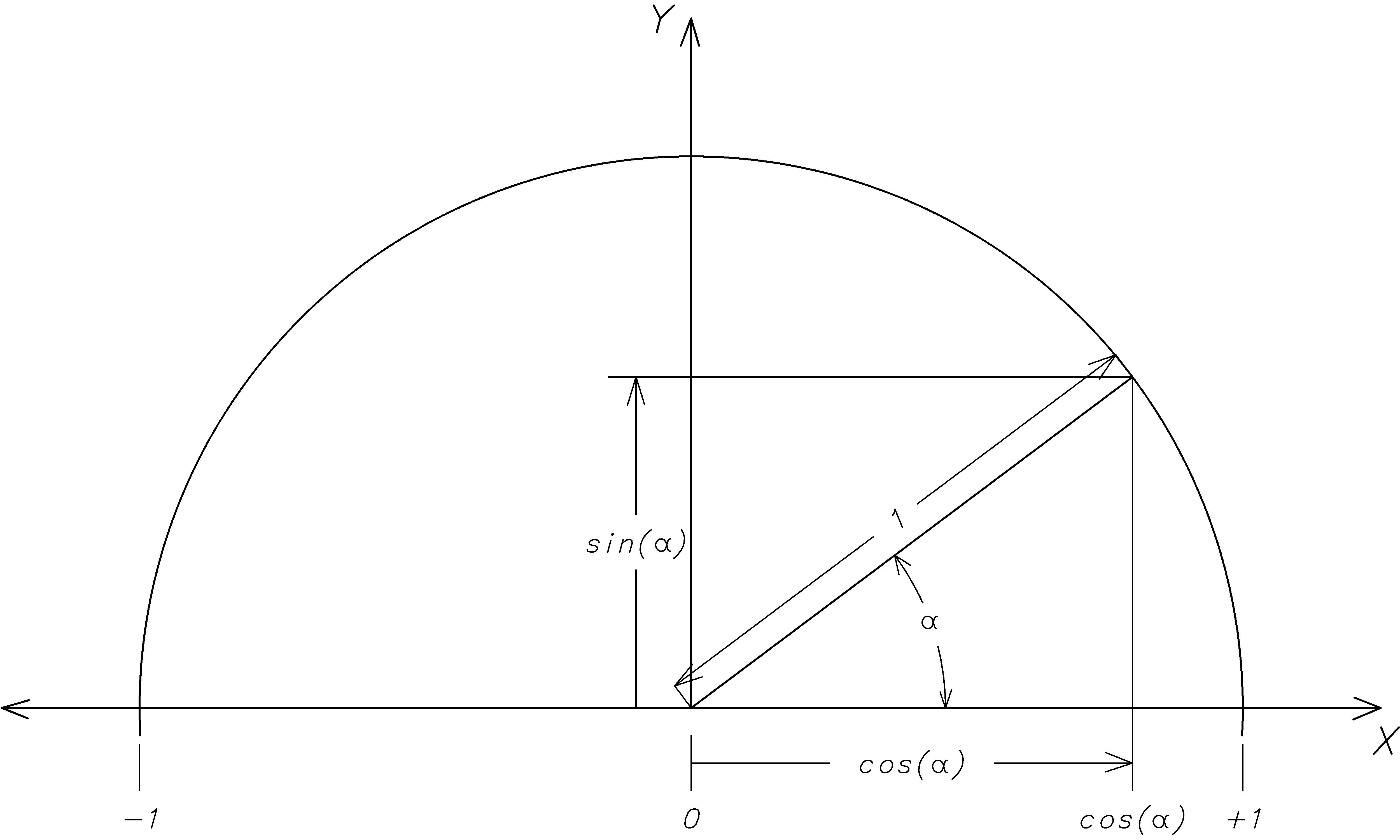
Let’s start with velocity↓↓↓, which is the change in position per change in time. This is a vector in the direction of the arrow from the starting position to the ending position. We’ll assume all the positions are in a vertical line (up and down) in order to ignore the vector direction, and concern ourselves only with the length of the distance between positions. Since we’ll measure position in meters, a difference in position is also some number of meters. Similarly, we’ll measure time in seconds, and a difference in time will be some number of seconds, giving a velocity in↓ meters per seconds↓↓ (m ⁄ s):
For example↓↓, if our rocket moves from a height of 0 meters straight up to a height of 0.003215 meters in 0.01 seconds, the velocity will be 0.3215 meters per second straight up. The magnitude (length, or size) of the velocity vector is known as the speed↓↓. In our example, we would say the speed of the rocket is 0.3215 m ⁄ s.
Acceleration↓↓↓ is the change in velocity per change in time. This (also a vector) is the difference in velocity over a period of time. Since we focus on motions only in the vertical direction, our velocities will also all be vertical. This simplifies addition and subtraction of velocity vectors to the addition and subtraction of their magnitudes (lengths, or speeds), with the corresponding direction being always either straight up or down (if we measure positive positions in the up direction, negative velocities will be down). Just as the difference between positions in meters is a number of meters, a difference in velocities of
meters per second is a number of
meters per second. Dividing again by seconds gives units of
meters per second per second. However, just as half of a half is one quarter (
(1 ⁄ 2) ⁄ 2 = 1 ⁄ 4),
per second per second is the same as
per second squared (
(1 ⁄ s) ⁄ s = 1 ⁄ s2). Thus, using the MKS system, acceleration
↓ has units of
meters per second squared↓↓ (
m ⁄ s2).
For example↓↓, if our rocket is moving with a velocity of 0.3215 m ⁄ s2 straight up at time 0.01 seconds, and is moving with a velocity of 0.6430 m ⁄ s straight up at time 0.02 seconds, then the corresponding acceleration is:
((0.6430 − 0.3215) m ⁄ s)/((0.02 − 0.01) s) = (0.3215 m ⁄ s)/(0.01 s) = 32.15 m ⁄ s2
Finally, we come to the measuring↓↓ of forces. Newton’s force equation↓ F = ma actually tells us how to measure forces. Using the MKS system: measure the acceleration of an object in meters per second squared (m ⁄ s2) and multiply by the mass of the object in kilograms (kg) to find the force vector↓↓ causing the acceleration. To honor the man that shared his insightful understanding of motion, physicists name the unit of force↓↓ that accelerates one kilogram of mass by one meter per second squared a Newton↓↓ (N). We can substitute the units into the force equation to write this as:
F = ma ⟶ N = (kg⋅m)/(s2)
For example, the force necessary to accelerate a 0.143 kg rocket 32.15 m ⁄ s2 is 4.59745 N, since 0.143⋅32.15 = 4.59745 and we are using MKS↓↓ units.
A trajectory↓ is the path of a projectile↓ (something that is thrown, fired, or launched). Before we start the rocket trajectory calculations, let’s try to get a feel for force in Newtons by considering a force we are all familiar with: the force of the earth’s gravity↓↓↓↓ that pulls objects down (towards the center of the earth).
Consider the force that a pound of chocolate would have in Newtons. First note that one pound (1 lb.) is a perfectly acceptable measure of force. Scales that measure the weight↓ of an object are measuring the force that the earth’s gravity exerts on the object, the pull down toward the ground that the object feels. An object’s weight↓ is a different from its mass↓. On the moon, the same object feels less pull down toward the center of the moon since the moon’s gravity is about 1/6th of the earth’s. The object’s weight on the moon is about 1/6th its weight on earth, even though its mass is the same. An object’s mass↓ is a measure of its inertia↓, the property of resisting acceleration (a change in motion). The more an object resists acceleration, the more mass it has, and a correspondingly greater force must be applied to change its motion.
Measuring force↓↓↓ with the weight of objects goes back to the 1700’s. Galileo’s famous experiments brought to light the fact that at sea level, the earth’s gravity accelerates↓↓ all objects at the same rate: approximately g ≈ 9.80665 m ⁄ s2. (This number changes as the distance from sea level changes.) Plugging this number for acceleration into the force equation, and 0.45359237 kg for the mass equivalent↓↓↓ to one pound of force↓ at sea level, we find the force in Newtons to be approximately 4.448 N. Alternatively, since 4.448 is between 4 and 5, one Newton feels like the force of between one quarter and one fifth of a pound.
F
=
m⋅a
=
m⋅g
4.448 N
≈
0.45359237 kg ⋅ 9.80665(m)/(s2)
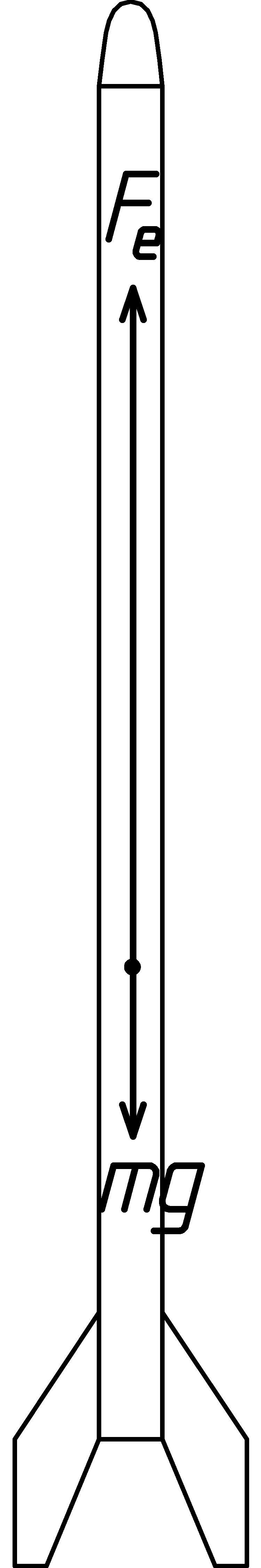
Now that we have some experience with force, mass, acceleration, and the force equation, let’s use them to see how a rocket shoots up through the sky. Our first step is to identify the forces acting on the rocket. Of course, gravity will pull the rocket down, but the rocket engine will push the rocket up. This lets us refine our force equation↓ by separating the total force F into the force of the rocket engine↓↓ Fe (using a plus sign since it pushes the rocket up) and the force of gravity↓↓ Fg = mg (with a negative sign since it pulls the rocket down) as follows:
F
=
ma
Fe − Fg
=
ma
Fe − mg
=
ma
Now divide both sides of the equation by the mass of the rocket to solve for the acceleration:
To generate trajectory estimates we’ll need some measurements. Let’s suppose that our rocket has a mass of 143 g. (This is the mass in grams reported for one of my model rockets by an electronic kitchen scale I use. The scale converts the gravitational force measured as the downward pull of the rocket into grams of mass using appropriate conversion factors that assume it is at sea level).
We’ll also need the engine thrust↓↓↓, the amount of pushing force of the engine. To do this, let’s suppose we choose a C6-3↓ engine. The C tells us that the engine will have a total mount of pushing power or total impulse↓↓ (amount of thrust for a period of time) in the range of 6 to 12 Newton-seconds. The Estes C6-3 engine has a total impulse of about 9 Newton-seconds. The 6 tells us that the average thrust will be about 6 Newtons, and the 3 tells us the (parachute deploying) final charge will have a delay↓ of about 3 seconds.
Plugging these numbers into our modified equation, we find the acceleration in units of m ⁄ s2:
a = (6 N)/(0.143 kg) − 9.80665 m ⁄ s2 ≈ 32.15 m ⁄ s2
We are almost ready to calculate how the rocket will move. However, in order to do so with the tools we have at hand, we must make the following simplifying assumption. Even though the height and velocity change rapidly with time, we will only look at the values at fixed points in time and assume these values remain relatively constant between time points. This approach is known as discrete sampling↓ and depends on values changing slowly along the sample points in order to yield accurate predictions.
We can now calculate how the rocket will move by starting with the rocket on the ground at an initial height of 0 meters, sitting still with an initial velocity of 0 meters/second. The only question remaining is what time unit to use. Since the velocity will be changing rapidly even though we’ll be assuming constant values over the time increment, the smaller the time increment, the more accurate will be our estimates. Let’s use a time increment of a hundredth of a second (0.01 seconds) to fill in the following table:
|
Time
|
Acceleration
|
Velocity
|
Height
|
|
(s)
|
(m ⁄ s2)
|
(m ⁄ s)
|
(m)
|
|
0.00
|
32.15
|
0.0000
|
0.0000
|
|
0.01
|
32.15
|
0.3215
|
0.0000
|
|
0.02
|
32.15
|
0.6430
|
0.003215
|
|
0.03
|
32.15
|
0.9645
|
0.009645
|
|
0.04
|
32.15
|
1.2860
|
0.019290
|
|
...
|
...
|
...
|
...
|
How did we get these numbers? We start with the idea that acceleration (32.15 m/s per second) is the change in velocity per second and multiply by the change in time of 0.01 seconds to get the change in velocity for that increment of time. We then add that velocity change to the entry in the velocity column for each time increment of 0.01 seconds. In a similar way, we use the idea that velocity is the change in height per second, and multiply the velocity by the change in time of 0.01 seconds to get the change in height.
For example, starting in the first row of the table, with an acceleration of 32.15 m ⁄ s2, a velocity of 0 m ⁄ s, we estimate that after 0.01 s the change in velocity will be 0.01 s⋅32.15 m ⁄ s2 = 0.3215 m ⁄ s. Since the acceleration is the same for the second row, the change in velocity will again 0.3215 m ⁄ s from row two to row three, giving a velocity of (0.3215 + 0.3215) m ⁄ s2 = 0.6430 m ⁄ s for the third row. At time 0.03 seconds, our velocity estimate will be (0.6430 + 0.3215) m ⁄ s2 = 0.9645 m ⁄ s. And so on.
Similarly, we can estimate the height of the rocket at the various times by using the estimated velocities. For example, after 0.01 s at a velocity of 0 m ⁄ s, there will be no change in height, so the height entry for time 0.01 seconds will be the same as for time 0.00 second, namely a height of 0 meters. However, with a velocity at time 0.01 seconds of 0.3215 m ⁄ s, we estimate the change in height from 0.01 seconds to 0.02 seconds as 0.01 s⋅0.3215 m ⁄ s = 0.003215 m, giving a height at time 0.02 seconds of 0.003215 m. In the same way, with a velocity at time 0.02 seconds of 0.6430 m ⁄ s, we estimate the change in height from 0.02 seconds to 0.03 seconds as 0.01 s⋅0.6430 m ⁄ s = 0.006430 m, giving a height at time 0.03 seconds of (0.003215 + 0.006430) m = 0.009645 m. And so on.
Notice that our assumption of constant, accurate values for a fixed time increment together with the procedure we use for generating estimates result in the peculiarity that initially the rocket does not move for two whole time increments regardless of the acceleration value. This is an artifact of our assumptions and procedures. To probe this issue further, try exercise 1↓.
Before going further, let’s stop and notice the patterns in the table. To do so, we’ll rewrite the table using a symbolic name for the increment in velocity. Since the acceleration is a constant 32.15 m ⁄ s2, so will the velocity increment↓ be a constant 0.3215 m ⁄ s as we saw above. We’ll give the symbolic name v to the increment 0.3215 and use it to rewrite the table as follows:
|
Time
|
Acceleration
|
Velocity
|
Height
|
|
(s)
|
(m ⁄ s2)
|
(m ⁄ s)
|
(m)
|
|
0.00
|
32.15
|
0
|
0
|
|
0.01
|
32.15
|
1v
|
0
|
|
0.02
|
32.15
|
2v
|
0.01v
|
|
0.03
|
32.15
|
3v
|
0.01(1 + 2)v
|
|
0.04
|
32.15
|
4v
|
0.01(1 + 2 + 3)v
|
|
...
|
...
|
...
|
...
|
More specifically, the velocity starts at 0 m ⁄ s, and to get the next velocity entry we simply add v to the current velocity. This results in a velocity entry that simply increments the number of v’s from each row to the next.
Similarly, the height starts at 0 m, and since the velocity is initially 0 m ⁄ s (not moving), to get the next height entry we add 0.01(0v) = 0 meters to the current one (0 meters). For the next entry (time 0.02), we multiply the previous velocity 1v by the time increment 0.01 and add it to the current height. At the next row (time 0.03) we add the contribution from 2v to the current row which already has the contribution of 1v, and so on. If you are still wondering how we got the last entry in the height column of the table, take a look at exercise 1↓.
Now let’s think about a particular, but generic, entry farther down in the table, the one for time 0.01n, without specifying n. It is pretty clear from our table and discussion above that just as 4v is the velocity for 0.04 seconds, the velocity estimate for time 0.01n seconds will be nv. We can also see that the corresponding height estimate will be 0.01(1 + 2 + 3 + … + (n − 1))v. This is a fine mathematical expression, but we can do a little better if we notice that pairs of numbers, one from the left and one from the right, sum to n. The final step is to notice how many pairs there will be. We have to be careful to consider both sequences with an even number of integers and sequences with an odd number. This is a good time to try exercises 1↓ and 1↓ to clarify this point so that you agree with the following calculation:
1 + 2 + 3… + (n − 3) + (n − 2) + (n − 1)
=
n + 2 + 3 + … + (n − 3) + (n − 2)
=
n + n + 3 + … + (n − 3)
=
…
n + n + n + …
=
(n(n − 1))/(2)
Using this summation trick, we can provide a general expression for the table of trajectory estimates for the powered part of flight as follows:
|
Time
|
Acceleration
|
Velocity
|
Height
|
|
(s)
|
(m ⁄ s2)
|
(m ⁄ s)
|
(m)
|
|
0.00
|
32.15
|
0v
|
0v
|
|
0.01
|
32.15
|
1v
|
0v
|
|
0.02
|
32.15
|
2v
|
0.01v
|
|
0.03
|
32.15
|
3v
|
0.01(1 + 2)v
|
|
0.04
|
32.15
|
4v
|
0.01(1 + 2 + 3)v
|
|
...
|
...
|
...
|
...
|
|
0.01n
|
32.15
|
nv
|
0.01n(n − 1)v ⁄ 2
|
|
...
|
...
|
...
|
...
|
How far should the table continue in this fashion? We can calculate how long the engine will supply thrust by dividing the total impulse↓ of the engine, 9 Newton-seconds for a C6-3 engine↓, by the average thrust of 6 Newtons to see that it should burn for about 1.5 seconds (that is, n = 150). What is the estimated height of the rocket at that point? What is the estimated velocity? Let’s plug in the value 150 for n and find out. We find that the velocity estimate for time 1.5 seconds is 150⋅0.3215 m ⁄ s = 48.225 m ⁄ s. Similarly, the estimated height at that time is 0.01(150⋅149)0.3215 m ⁄ 2 = 35.927625 m.
What happens when the rocket engine cuts out? Look back to the equation for acceleration on page 1↑. When Fe goes to zero, the equation becomes: − g = a. Once the engine thrust stops, the only remaining force acting on the rocket is the downward pull of earth’s gravity, reducing the upward velocity with its downward acceleration. This is called the coast phase↓ of the flight in contrast to the previous powered phase↓ when the engine is thrusting. We’ll assume that the rocket is near enough to the surface of the earth to use the same gravitational acceleration↓↓ g = 9.80665 m ⁄ s2 throughout. We can calculate estimates just as we did before, except that now we use a downward acceleration, negative 9.80665 m ⁄ s2. We’ll start a new table at the point the engine dies, starting from our results above, adding 0.01( − 9.80665) m ⁄ s = − 0.0980665 m ⁄ s to each subsequent velocity entry, and adding the product of velocity and 0.01 s for each subsequent height entry:
|
Time
|
Acceleration
|
Velocity
|
Height
|
|
(s)
|
(m ⁄ s2)
|
(m ⁄ s)
|
(m)
|
|
1.50
|
-9.80665
|
48.225
|
35.927625
|
|
1.51
|
-9.80665
|
48.1269335
|
36.409875
|
|
1.52
|
-9.80665
|
48.0288670
|
36.891144335
|
|
1.53
|
-9.80665
|
47.9308005
|
37.371433005
|
|
1.54
|
-9.80665
|
47.8327340
|
37.850741010
|
|
...
|
...
|
...
|
...
|
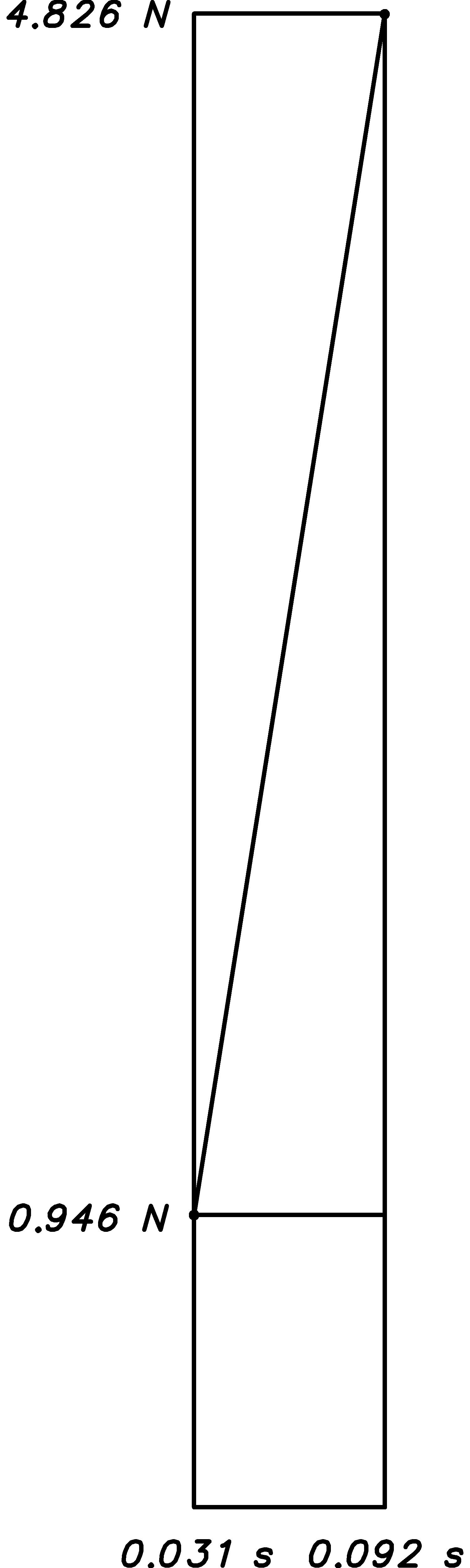
Just as before, we’re interested in the patterns that form the numbers. We’ll introduce some symbols so that we end up with algebraic expressions for the entries. That way, we’ll be able to plug different values in, and even solve for values that are interesting to us, as we shall see. Let’s start by introducing a symbolic name d for the velocity increment↓ 0.0980665, and rewrite the table with it instead of the numeric values as follows:
|
Time
|
Accel.
|
Velocity
|
Height
|
|
(s)
|
(m ⁄ s2)
|
(m ⁄ s)
|
(m)
|
|
1.50
|
-9.80665
|
48.225
|
35.927625
|
|
1.51
|
-9.80665
|
48.225 − d
|
35.927625 + 0.01(48.225)
|
|
1.52
|
-9.80665
|
48.225 − 2d
|
35.927625 + 0.01(2⋅48.225 − d)
|
|
1.53
|
-9.80665
|
48.225 − 3d
|
35.927625 + 0.01(3⋅48.225 − (1 + 2)d)
|
|
1.54
|
-9.80665
|
48.225 − 4d
|
35.927625 + 0.01(4⋅48.225 − (1 + 2 + 3)d)
|
|
...
|
...
|
...
|
...
|
This is a good time to verify the height entries in the last column of the table by trying exercise 1↓ before going on.
Now continue by introducing symbolic names T, V, and H for the starting time, velocity, and height respectively, and rewrite:
|
Time
|
Acceleration
|
Velocity
|
Height
|
|
(s)
|
(m ⁄ s2)
|
(m ⁄ s)
|
(m)
|
|
T
|
-9.80665
|
V
|
H
|
|
T + 0.01
|
-9.80665
|
V − d
|
H + 0.01(V)
|
|
T + 0.02
|
-9.80665
|
V − 2d
|
H + 0.01(2V − d)
|
|
T + 0.03
|
-9.80665
|
V − 3d
|
H + 0.01(3V − (1 + 2)d
|
|
T + 0.04
|
-9.80665
|
V − 4d
|
H + 0.01(4V − (1 + 2 + 3)d)
|
|
...
|
...
|
...
|
...
|
Just as before, we’ll focus our attention on an entry lower in the table, say, for time T + 0.01k. Once again, we can see from the table that the velocity entry at time T + 0.01k will be V − kd, and the height entry will be H + 0.01(kV − (1 + 2 + 3 + … + (k − 1))d). Using our summation trick again, we can write the sum 1 + 2 + 3 + … + (k − 1) as (k(k − 1) ⁄ 2) so that the table of trajectory estimates for the coasting phase of the flight becomes:
|
Time
|
Acceleration
|
Velocity
|
Height
|
|
(s)
|
(m ⁄ s2)
|
(m ⁄ s)
|
(m)
|
|
T
|
-9.80665
|
V
|
H
|
|
T + 0.01
|
-9.80665
|
V − 1d
|
H + 0.01(V)
|
|
T + 0.02
|
-9.80665
|
V − 2d
|
H + 0.01(2V − (1)d)
|
|
T + 0.03
|
-9.80665
|
V − 3d
|
H + 0.01(3V − (1 + 2)d)
|
|
T + 0.04
|
-9.80665
|
V − 4d
|
H + 0.01(4V − (1 + 2 + 3)d)
|
|
...
|
...
|
...
|
...
|
|
T + 0.01k
|
-9.80665
|
V − kd
|
H + 0.01(kV − k(k − 1)d ⁄ 2)
|
|
...
|
...
|
...
|
...
|
What does this table actually tell us? The first thing to notice is that the velocity will remain positive (the rocket will continue its upward climb) until kd becomes larger than V. When does this happen? Plug the numbers for V and d into V − dk = 0 and solve for k! Once we know k, we have an estimate for how long the rocket will climb, coasting after the engine dies. We can use this time estimate to pick an engine with a similar delay so that the rocket will go as high as possible and its velocity will be small when the parachute is deployed. The highest point of the climb is called the apogee↓. We can estimate the apogee by plugging the numbers for T, V, H, d, and k into H + 0.01(kV − k(k − 1)d ⁄ 2). If we want to estimate the height with a 3 second engine delay↓ for deployment of a parachute, plug in a corresponding value for k. (A 3 second delay gives a k of 300.)
Before you get too excited about these rocket trajectory estimates, let me give you a clue to an improvement we’ll work on in the next chapter. Anyone who has ridden a bike against a strong wind will know that we are ignoring a significant component that will affect our height estimate for the rocket. Before we get to it, however, give the following exercises a try.
Exercises
-
Use the acceleration equation on page 1↑ to find the acceleration a for a 0.143 kilogram rocket using a C11-X engine (having average thrust of 11 Newtons). What is the corresponding 0.01 second velocity increment v for this constant acceleration?
-
What arithmetic laws do we use to rewrite the sum 0.01v + 0.01(2v) + 0.01(3v) as 0.01(1 + 2 + 3)v? List the steps in between and justify each step with an arithmetic law.
-
Verify visually that 1 + 2 + … + 7 = 8⋅7 ⁄ 2 by: writing out the list of numbers, connecting the first and last numbers, then the 2nd and 2nd to last, and so on, counting the number of lines you draw. Do the same for 1 + 2 + … + 8 = 9⋅8 ⁄ 2.
-
Verify visually that 1 + 2 + … + 7 = 8⋅7 ⁄ 2 by: writing out the list of numbers and its reverse so that the smallest of the 1st list pairs with the largest of the 2nd, the next smallest of the 1st pairs with the next smallest of the 2nd, and so on. What is the sum of each pair? How many pairs are there?
-
Show that: 0.01(48.225) + 0.01(48.225 − d) + 0.01(48.225 − 2d) + 0.01(48.225 − 3d) is the same as 0.01(4⋅48.225 − (1 + 2 + 3)d by listing the steps in between and justifying each step with an arithmetic law.
-
Find the number n of 0.01 second increments before the C11-X engine (9.0 Newton-seconds total↓ impulse) cuts out. Use this and the 0.01 second velocity increment v from exercise 1↑ to determine the velocity V = nv, and height H = 0.01n(n − 1)v ⁄ 2 at the time the engine dies.
-
Use the values V = 48.225 m ⁄ s and d = 0.0980665 m ⁄ s in the equation V = kd we found in the text to calculate the number of 0.01 second increments k until apogee. Use this value to find the coast time as k⋅0.01 s. Finally, calculate the apogee as H + 0.01(kV − (k − 1)(k − 2)d ⁄ 2) using the value H = 35.927625 m from the text.
-
Use the value of V from exercise 1↑ and d = 0.0980665 m ⁄ s in the equation V = kd we found in the text to calculate the number of 0.01 second increments k until apogee. Use this value to find the coast time as k⋅0.01 s. Finally, calculate the apogee as H + 0.01(kV − (k − 1)(k − 2)d ⁄ 2) using the value of H from exercise 1↑.
-
Assume that your rocket deploys a very large parachute that will essentially stop the rocket from moving (pulls very strongly, stopped relative to a fast velocity). Say your rocket has a mass of 200 grams and and is moving at 50 meters per second. What is the force in Newtons that your rocket will exert on the parachute? What is the force in pounds? [Hint: Divide the number of Newtons by 4.448 Newtons per pound to get the force in pounds.] What does this say about the sturdiness of your parachute and attachment? In what way can we reduce the forces on the parachute?
-
Explain how the force equation can be used to define↓ and measure↓ mass.
-
We are really on to something with the observation from page 1↑ that T + 0.01k represents the time for the kth entry in the trajectory estimate table on page 1↑. In this exercise, you’ll rewrite the symbolic expressions for both the velocity, V − kd, and the height, H + 0.01(kV − k(k − 1)d ⁄ 2), as follows:
-
Substitute 0.01a for − d in the expressions for velocity and height.
-
Regroup the values in the results of (a) so that 0.01 and k always appear together as 0.01k.
-
Substitute t for 0.01k in the results of (b).
-
Regroup the the results of part (c) into the form Mt + B for velocity, and At2 + Bt + C for height. We call the values M, B, A, and C coefficients↓ of the various powers of t.
-
The points satisfying the equation y = Mx + B form a line↓↓ and often result from a quantity y that changes in proportion M to some other quantity x. We say that the function y is linear↓↓ in x. Which of the following trajectory quantities is linear in time t: height, velocity, and/or acceleration?
-
The points satisfying the equation y = Ax2 + Bx + C form a parabola↓↓ and often result from a quantity y that accumulates↓ (adds up) values that are linear in a quantity x. We say that the function y is quadratic↓↓ in x. What trajectory quantity is quadratic in time t? What trajectory quantity linear in t is being accumulated?
-
The coefficient B in the quadratic expression for height from part (d) should contain the term: 0.01a ⁄ 2. As we make our time increment 0.01 smaller and smaller, the values for a and t will remain the same, but what happens to the term: 0.01a ⁄ 2? This term is an artifact of the assumptions and the procedures we used to calculate the trajectory values. Rewrite the quadratic height expression from part (d) for the case of a time increment so small that we can leave out the term: 0.01a ⁄ 2.
2 Drag
Let’s say our rocket is moving at a speed of 48.225 m ⁄ s. That’s almost 108 miles per hour (see exercise 1). That’s pretty fast. If you’ve ever stuck your hand outside a fast moving vehicle, you’ve actually felt how hard the air pushes back against fast moving objects. In the field of fluid mechanics this force is called drag↓ and if we want to accurately estimate the trajectory of our rocket, we’ll have to incorporate it into our calculations.
If we think about it a bit, we’ll be able to come up with a sensible term to add to our force equation. For instance, you may have noticed from your fast moving experiences that the faster you move (assuming the air is more or less still), the more force you feel from the air. In other words, the resistance↓ will oppose your motion and increase with increasing velocity (denoted as v). The simplest expression that captures this is − Cv for some constant C, but is this really all we need? What else effects the strength of the wind pushing on an object? Think about flying a kite.
Other important factors are the size and shape of the object. The more surface area A pressing directly into the air (we’ll call this drag surface area↓), the greater the resistance. This is why a parachute slows a fall to a non-destructive speed. Along with the drag surface area, our drag force term should also include a constant factor known as the drag coefficient↓ CD that captures the shape and texture of the surface moving against the air, varying from near 0 for a polished, smoothly curved, streamlined body that cuts through the air up to about 2 for a rough flat plate perpendicular to the motion.
A simple expression incorporating these factors is − ACDv, but there is still more to consider. Let’s think about the air. Air is a fluid that flows and has density↓↓. It flows freely (low viscosity), so we will not need to account for the viscosity↓↓ of the air (as we would for a thick, viscous substance such as honey). Density↓ is the mass of a substance per unit volume. It measures↓↓↓↓ the concentration of mass and, expressed in MKS units, we’ll use it in the form of kilograms per meter cubed (kg ⁄ m3) . The greater the density, the more a fluid resists motions through it (in the F = ma, push-and-shove sort of way that it is difficult to run through a pool). Density will vary with altitude, which will (hopefully) change rapidly along the rocket trajectory, so we’ll include air density as the factor ρ(h) (using functional notation that reminds us that the density ρ will vary with height h). Our reasoning thus far yields the following drag force expression: − ρ(h)ACDv, however ...
One final consideration will shape our drag force term. We will base our reasoning on dimension analysis. Dimension analysis↓ is based on the principle that expressions should have the proper measurement units. For instance, the drag force term should have units of force: Newtons. We start with a drag term that includes the factors we’ve already mentioned, leaving the velocity part a bit general:
In other words, rather than including velocity directly as v, we include some function of velocity f(v), that could be linear, quadratic, or even more complicated in order to make the whole drag force come out in units of force (Netwons). Hopefully, this intuitively makes sense so far: twice as much drag surface area gives twice as much resistance to motion. The same goes for density: twice as much density gives twice as much resistance to motion. The drag coefficient is just a knob that we dial up to 2 for surface shapes that catch the wind, and down to 0 for shapes that glide through the air freely.
Now comes the tricky part. If we measure↓↓ air density↓ in units of kg ⁄ m3, drag surface area in m2, and make CD dimensionless (no units, just a number), leaving aside for the moment the units of f(v), then the product of units so far is:
− ρ(h)CDAf(v) ⟶ (kg)/(m3)⋅m2⋅? = (kg)/(m3m)⋅?
However, we want our drag term to be a force and have units of force. Specifically, we want the units to be Newtons, or equivalently, kg⋅m ⁄ s2. So we have kg ⁄ m, but we want kg⋅m ⁄ s2 and we haven’t yet taken into account the factor f(v). However, since we measure velocity in units of m ⁄ s, when we multiply by some power of velocity v, we multiply the units by a power of m ⁄ s. It is now easy to see that we can get units of force by changing f(v) into v2, multiplying kg ⁄ m by m2 ⁄ s2. Furthermore, we follow a convention in fluid mechanics of introducing the factor of 1 ⁄ 2 to make the velocity factor v2 ⁄ 2 look like a kinetic energy↓ term without the mass. Thus, our final drag term becomes:
This drag term↓ is the improvement we’ve been looking for. When we add it into our modified force equation from the last chapter, our new and improved force equation↓ becomes:
Fe − mg − ρ(h)CDA(v2)/(2) = ma
Once we solve for acceleration, we can use the resulting equation the same way we did in the last chapter, only with even more accurate results. Let’s divide through by the mass of the rocket to find out how to calculate the acceleration:
(Fe)/(m) − g − (ρ(h)CDAv2)/(2m) = a
What to do about the air density? Rather than go into all of that right now, let’s simplify and assume a constant air density near ground level of↓↓ approximately 1.2 kg ⁄ m3. As we generate numbers, we’ll have to keep in mind that the drag will be slightly less than calculated as the rocket climbs higher, since air density deceases with increasing altitude.
To calculate the drag acceleration for our rocket from chapter 1↑ we’ll need the drag surface area, which is approximately 0.00226356 m2 (see exercise 2), and we’ll guesstimate the drag coefficient as 0.7 (close to the value for a long cylinder, but somewhat more streamlined). This yields the following drag acceleration term
( − ρ(h)CDAv2)/(2m) ≈ ( − 1.2(0.7)(0.00226356))/(2(0.143))v2 ≈ − 0.0066482v2
We are finally ready to generate some numbers. We’ll add another column to the table to help us keep track of the contribution of the drag term and round off values at 4 decimal places:
|
Time
|
Fe ⁄ m − g
|
− ρ(h)CDAv2 ⁄ 2m
|
a
|
v
|
h
|
|
(s)
|
(m ⁄ s2)
|
(m ⁄ s2)
|
(m ⁄ s2)
|
(m ⁄ s)
|
(m)
|
|
0.00
|
32.1514
|
0.0000
|
32.1514
|
0.0000
|
0.0000
|
|
0.01
|
32.1514
|
0.0000
|
32.1514
|
0.3215
|
0.0000
|
|
0.02
|
32.1514
|
-0.0007
|
32.1407
|
0.6430
|
0.0032
|
|
0.03
|
32.1514
|
-0.0027
|
32.1486
|
0.9645
|
0.0096
|
|
0.04
|
32.1514
|
-0.0062
|
32.1452
|
1.2860
|
0.0193
|
|
...
|
...
|
...
|
...
|
...
|
...
|
|
0.50
|
32.1514
|
-1.5999
|
30.5515
|
15.8190
|
3.9085
|
|
...
|
...
|
|
|
...
|
...
|
|
1.48
|
32.1514
|
-11.3142
|
20.8372
|
41.4630
|
32.6395
|
|
1.49
|
32.1514
|
-11.4295
|
20.7219
|
41.8786
|
33.0542
|
|
1.50
|
-9.8066
|
-11.5446
|
-21.3513
|
41.8786
|
33.4709
|
|
1.51
|
-9.8066
|
-11.6597
|
-21.4664
|
41.6651
|
33.8897
|
|
1.52
|
-9.8066
|
-11.5411
|
-21.3478
|
41.4504
|
34.3063
|
|
...
|
...
|
|
|
...
|
...
|
|
4.73
|
-9.8066
|
-0.0001
|
-9.8068
|
0.0339
|
92.3012
|
|
4.74
|
-9.8066
|
0.0000
|
-9.8067
|
-0.0642
|
92.3015
|
|
4.75
|
-9.8066
|
0.0000
|
-9.8066
|
-0.1622
|
92.3008
|
|
4.76
|
-9.8066
|
0.0002
|
-9.8065
|
-0.2603
|
92.2992
|
|
...
|
...
|
|
|
...
|
...
|
With this table of numbers before us, let me point out a few interesting properties. First and foremost we notice that the drag↓ contribution does indeed increase at higher velocities, reducing the acceleration by over a third. At maximum velocity the effect on velocity is not that pronounced, only about 20 percent. However, the overall effect of drag on the apogee (maximum height) through the reduced velocity is dramatic. Chapter 1 exercise 1↑ asks you to calculate the apogee without drag, giving a value close to 154.75 meters. Here we find a value close to 92.3 meters, about 60% of the value without drag. The velocity reduction of 20% accumulates to make a dramatic 60% difference in the maximum height.
Next notice the apogee↓ values, predicted to occur sometime near 4.74 seconds. The velocity is so small, with relatively small acceleration, that the rocket seems to just hang in the air for a moment. Furthermore, as the velocity crosses from positive to negative, the drag contribution crosses from negative to positive, a sort of secondary effect to reduce acceleration and thereby resist motion. The increasing drag would be important if we wanted to know (see exercises 2↓ and 2↓) how long the rocket would take to hit the ground without a parachute, streamer, or other mechanism to slow the fall, but this is something we try to avoid so that we don’t break anything (including the rocket). This brings us to the next key point: the apogee occurs approximately 4.74 − 1.50 = 3.24 seconds after the engine burn cuts off, so that a 3 second delay↓ is just about right for parachute deployment (or other drag increasing mechanism). The time from engine cut-off until apogee is known as coast time↓. We want to match the rocket engine delay as closely as possible to the coast time to achieve maximum height and avoid damaging the parachute. See exercise 1↑ of chapter 1↑.
Finally, let’s talk about calculating all these numbers. While it is theoretically possible to calculate them all by hand (or with a handheld calculator), my personal preference is to set up a spreadsheet to do it all, though you could also write a program to generate them. In the next chapter we’ll take a look at creating a spreadsheet to automate the calculations, but first, try your hand at some of the following exercises.
Exercises
-
Use the following unit equivalences to convert↓ 48.225 m ⁄ s into units of miles per hour (mph).
100 cm
=
1 m
2.54 cm
=
1 in
12 in
=
1 ft
5280 ft
=
1 mi
60 s
=
1 min
60 min
=
1 hr
[Hint: Let’s look at a conversion↓ of 100 cm into feet. Since 2.54 cm = 1 in, and 12 in = 1 ft, we know that 1 = 1 in ⁄ 2.54 cm, that 1 = 1 ft ⁄ 12 in and that we can always multiply anything by 1 and keep it equal to itself, so we can multiply in a way that units cancel, converting cm to ft as follows:
100 cm⋅(1 in)/(2.54 cm)⋅(1 ft)/(12 in) = (100)/(2.54⋅12)ft
Use the same idea to convert 48.225 m ⁄ s by converting both meters to miles and seconds to hours all in one long product of velocity and conversion factors.]
-
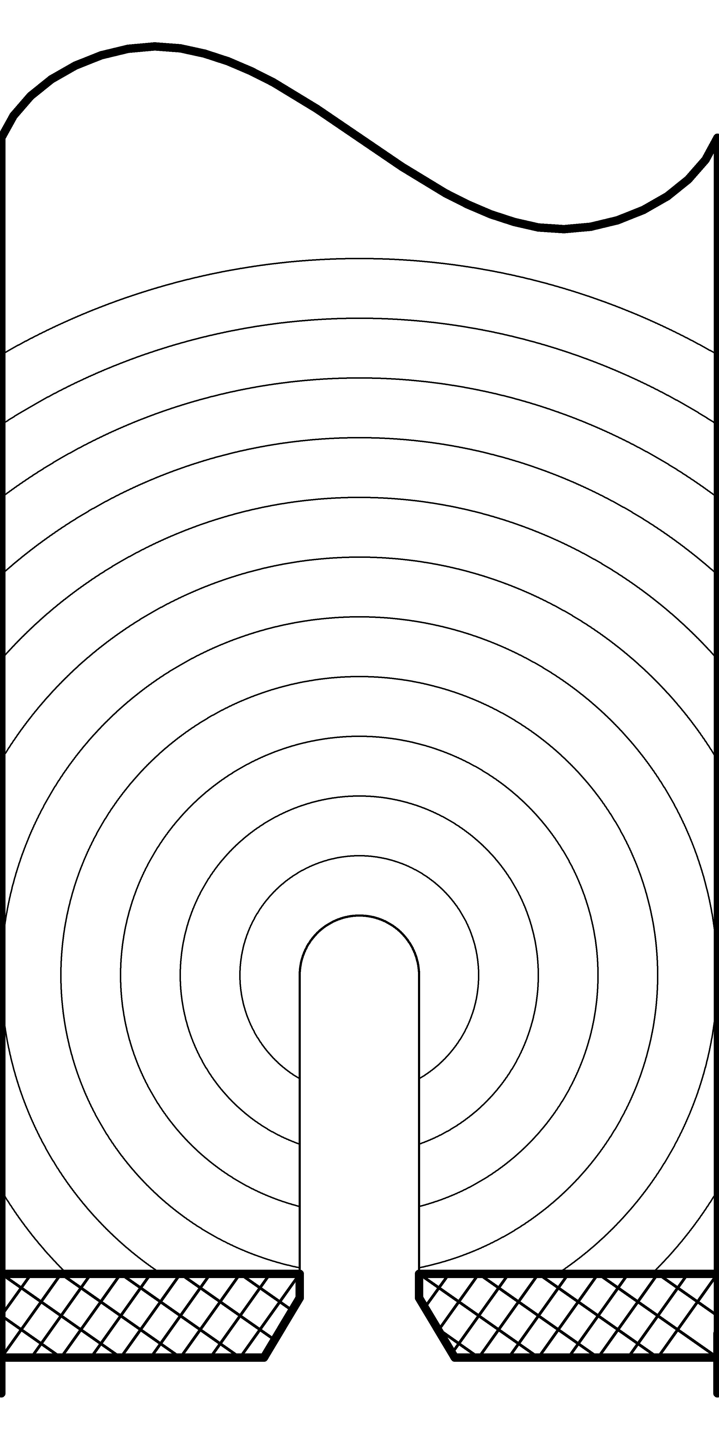
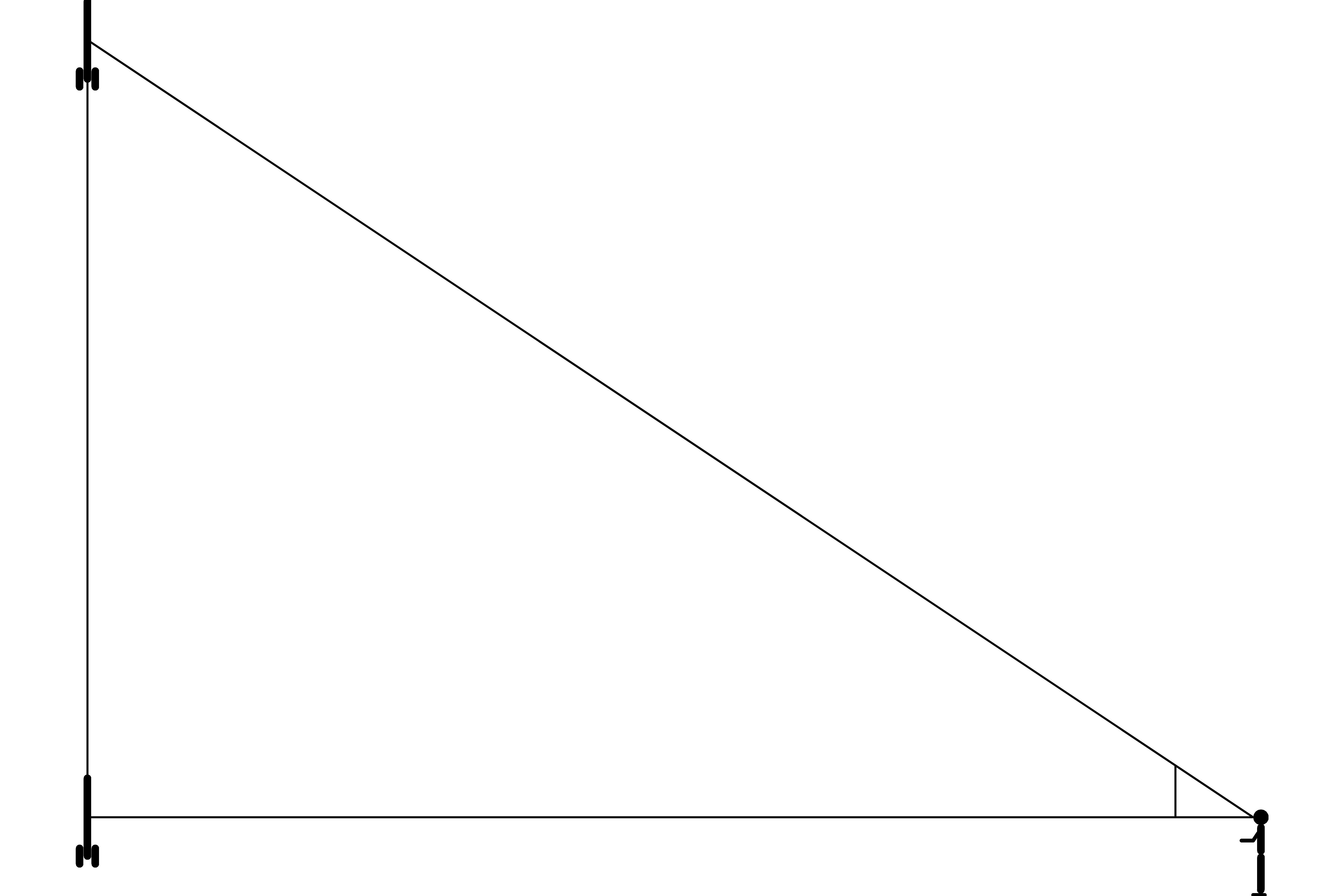
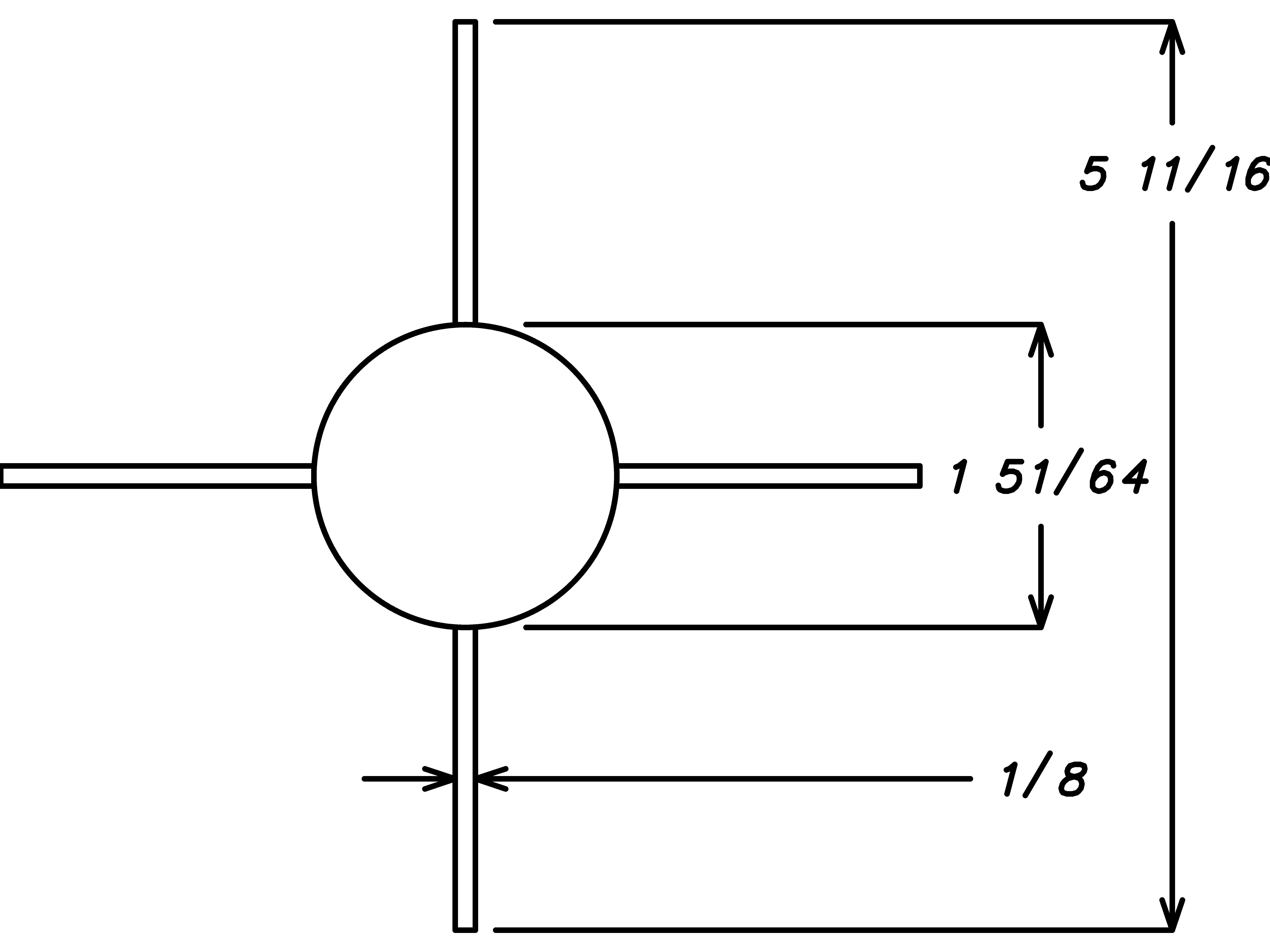
Calculate the area of a rocket that has a cylindrical body with a diameter of 1 + 51 ⁄ 64 in with 4 fins that measure 1 ⁄ 8 in thick and would make a 5 + 11 ⁄ 16 in diameter circle if you rotated the rocket around its body-cylinder axis (see the diagram on the next page). [Hint: The area of a circle is πr2. To convert square inches into square centimeters, multiply by (2.54 cm ⁄ in)2. To convert square centimeters to square meters, multiply by (1 m ⁄ 100 cm)2.]
-
Suppose a rocket with a drag surface area A = 0.00226 m2 and a drag coefficient CD = 0.7 is moving with a velocity v = 42.086 m ⁄ s. Using an air density ρ = 1.2 kg ⁄ m, calculate our estimate of the drag force ρCDAv2 ⁄ 2. Now divide by the rocket mass m = 0.143 kg to find the corresponding acceleration.
-
Suppose you make a small change in the shape of the rocket that reduces the drag coefficient by 10%. Do you think the effect on maximum velocity will be greater than, less than, or equal to 10%? Why? How about the effect on apogee? Why?
-
Noticing from the table on page 1↑ that the rocket is expected to coast for about 3.24 seconds from a velocity of approximately 42 m ⁄ s, do you think the speed of the rocket would be more, equal, or less than about 42 m ⁄ s after falling for 3.24 seconds without a parachute (or similar device)? Why? [Hint: Consider the acceleration on the way up and the way down. Is it the same?]
-
There is an interesting condition for the velocity that occurs when the drag exactly cancels the gravitational force pulling the rocket down. We call this the terminal velocity↓↓.
-
What can you say about the change in velocity of the falling rocket at terminal velocity?
-
Write an equation that sets the drag force term equal to the gravitational force pulling the rocket down by equating the gravitational force − mg to the drag force ρCDAv2 ⁄ 2 (on the way down there is no minus sign since the drag pushes up).
-
Plug the numbers from the text into the equation.
-
Solve the equation in part (c) by manipulating the equation to first get v2 by itself on one side of the equation, then take the square roots of both sides to solve for v. Make sure you include measurement units in the equation and carry them all the way through so that you have meaningful units for the terminal velocity solution.
-
How would increased humidity affect the drag?
3 Automate via Spreadsheet
In order to be able to automate calculations, check results, and recognize and fix problems, it really is necessary to understand the calculations involved with trajectory estimations, and to do enough of them by hand that you get a good feeling for what is going on. However, when you have a set of thousands of detailed calculations that change each time you change a parameter, there is no substitution for some sort of automation such as a spreadsheet. Think of a spreadsheet as a special purpose programming language designed specifically for organizing, calculating, and displaying numbers in the easiest general-purpose way possible. Rather than just leave you to it, discovering the highlights and pitfalls on your own, I’d like to offer the following advice to help you get started.
I’ll try to keep the discussion here at the right level, but if it seems that I’m overstating the obvious feel free to skim the text (or skip it altogether) and get down to the business of automating your trajectory estimates. On the other hand if it seems that I am going too fast or talking in gibberish without explaining what’s going on, you may have to ask someone for help, crack open either a spreadsheet manual or tutorial, then come back here and give it another go.
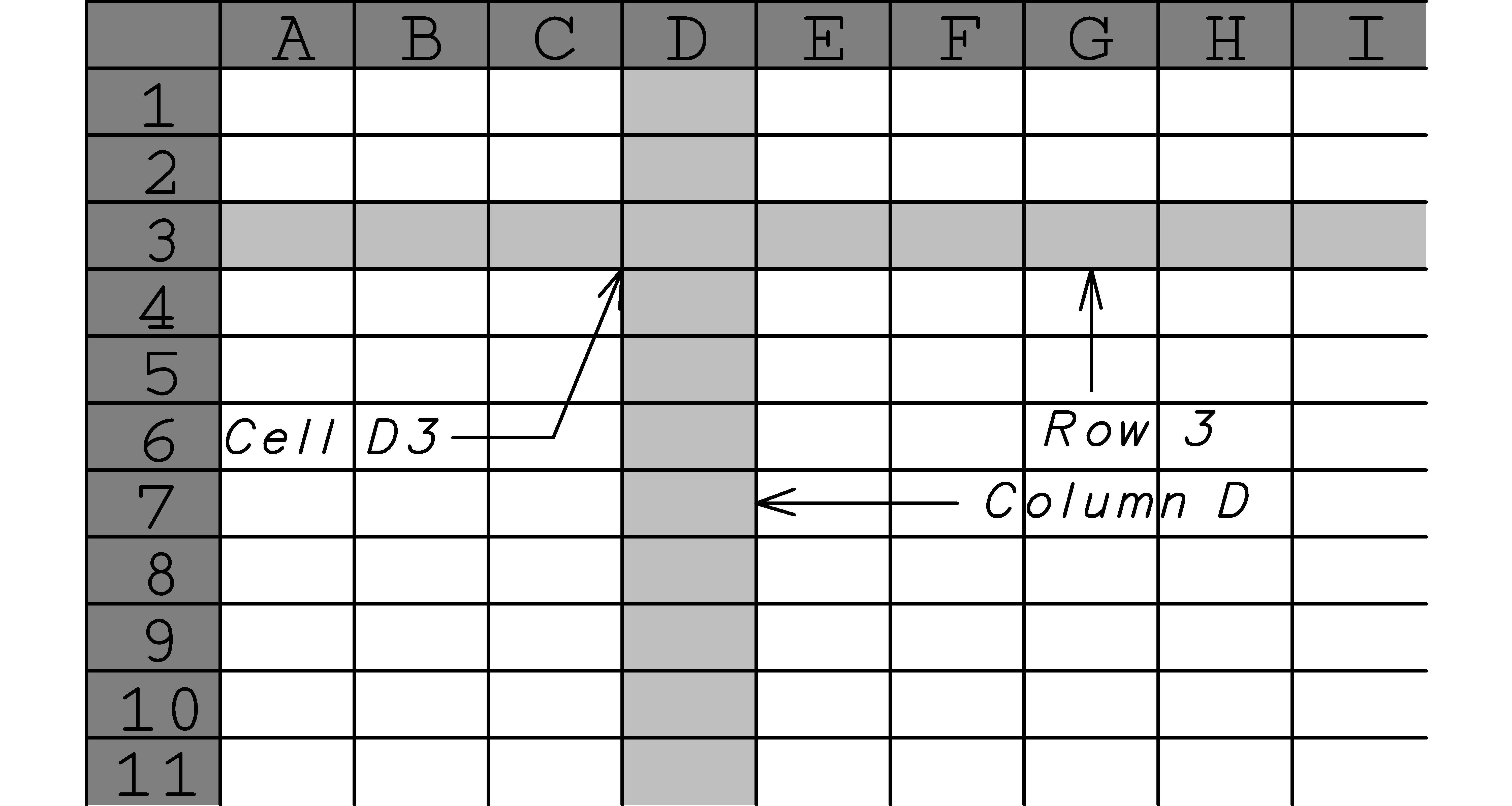
At the most basic level, a spreadsheet↓ is a matrix (a two dimensional table of rows and columns) of cells. The rows↓ are labeled with numbers, starting with 1 in the top-most row, and the columns↓ are labeled with letters, starting with A in the left-most column. Each cell↓↓ is specified with a column and row, such as D3, and can display either text or a numeric value. You can think of each numeric cell↓↓ as a calculator that can hold either a number, or the result of a calculation specified by a formula.
Formulas↓↓ can
reference↓↓↓ (use the numeric values from) other cells in the spreadsheet. For example, you can enter a formula into cell C3 that adds the values of cells A1 and B2 by moving the cursor over the C3 cell, left-clicking it, and typing in: =A1+B2. This cell will now display the sum of the numeric values of cells A1 and B2. Changing the value in cell A1 or B2 will change the result that is displayed in cell C3. Other cells can use the value cell C3 for their calculations. This is a good point to do exercises
8↓ and
8↓ to familiarize yourself with what we’ve covered so far if you haven’t used spreadsheets before, or you’ve only used one a few times and you’d like to practice.
Now, let’s talk about the different kinds of cells that we’ll use to organize our spreadsheet and calculations. There will be input cells↓↓↓, where we enter numbers that we’ve measured (such as the mass of the rocket in grams, diameter of the body in inches), or text values that we’ll use to specify information (such as the name of the rocket or the type of engine (C6-3)). It will also be useful to have pre-processed inputs, results of conversions or recombinations of inputs, that we’ll call derived input cells↓↓↓ containing such things as drag surface area, and rocket mass. Next, we’ll have the trajectory calculation cells↓↓↓ that generate various numbers that form the trajectory estimates using spreadsheet formulas. In addition we’ll have post-processing cells containing spreadsheet formulas to calculate important results such as apogee, maximum velocity and such, that we’ll call output cells↓↓.
In addition, to help ourselves and others use the spreadsheet, we’ll use comment cells↓↓ containing either formatting text or useful information about the spreadsheet. Furthermore, to make things even easier, we’ll color the background of cells depending on their type. The scheme I use is green for input cells, yellow for derived input cells, orange for output cells, clear background (white) for comment and intermediate calculation cells, and gray for headings and titles.
Before we go any farther, I should also say a couple of things about specific spreadsheet programs since they differ slightly. The instructions in the chapter work with the Gnumeric spreadsheet, version 1.8.2. However, the same instructions should also work with either Microsoft Excel, or OpenOffice Calc with the following differences that matter to us:
-
Function names in Gnumeric are in lower case, but in Excel and Calc are in upper case.
-
Function parameters are separated with commas in Gnumeric and Excel, but with semicolons in Calc.
-
The vlookup()↓ spreadsheet function↓ in Gnumeric has an optional 5th parameter that Excel doesn’t, but we don’t use it anyway. We’ll look at this function more closely in the Derived Inputs section below.
For example, we’d enter a formula such as =sum(A1,A2,C3:C5) for Gnumeric, but for Excel we’d enter =SUM(A1,A2,C3:C5), and for Calc we’d enter: =SUM(A1;A2;C3:C5).
Input Cells
It is better to keep the input cells↓↓↓ in the upper left part of the spreadsheet, the default home↓ position, because this is the area that will show up in the window when you open the spreadsheet. On the next page is an example of what I am talking about and we’ll go through it all in detail below, but first let me explain about the antiquated inches measuring units.
Most of my measurement tools are from my wood-shop where I do most of my measuring in inches and fractions of inches. However, this being a spreadsheet, meters or centimeters or whatever, are only a short conversion away (take a look back at exercise 2↑ in chapter 2↑). Furthermore, a measurement such as 1+51/64 inches can be entered just as it is typed, provided you precede it with an equals sign (=) to tell the spreadsheet you are entering a numeric↓ expression. It will then show up in the spreadsheet as 1.797 if the cell is formatted to show 3 digits of precision.
|
Rocket Trajectory Estimation Spreadsheet
|
|
|
|
|
|
|
|
|
|
|
|
|
Rocket Properties
|
Fins
|
Drag
|
|
|
Mass
|
Drag
|
Body
|
Num
|
Thick
|
Dia
|
Area
|
Area
|
|
Name
|
(g)
|
Coeff
|
Dia (in)
|
|
(in)
|
(in)
|
(in^2)
|
(m^2)
|
|
RedPhoenix
|
143
|
0.700
|
1.797
|
4.000
|
0.125
|
5.688
|
|
|
|
RedDevil
|
283
|
0.700
|
1.797
|
4.000
|
0.125
|
5.688
|
|
|
|
|
|
|
|
|
|
|
|
|
|
|
|
|
|
|
|
|
|
|
|
|
|
Flight Combination
|
Trajectory Constants
|
|
RedPhoenix
|
Rocket
|
|
1.20000
|
Air Density (kg/m^3)
|
|
EstesC6
|
Engine
|
|
9.80665
|
Gravitational Acceleration (m/s^2)
|
|
|
|
|
|
0.01000
|
Time Increment (s)
|
|
|
|
|
|
9.00000
|
Total Impulse (Ns)
|
|
|
|
|
|
6.00000
|
Average Thrust (Ns)
|
|
|
|
|
|
|
|
|
|
|
|
Let me say a few words about formatting↓↓↓↓. In order to have your table look like the one in this pamphlet, you’ll need to do some formatting. First, from the main menu, select Format, then Column, then Standard Width and enter the value 66 (points). Next, with the Rocket Properties table rows starting at cell A6 and extending though cells I9 (we write this cell range↓↓ as A6:I9), select↓↓ the cell range D6:I9 as follows. Move the cursor over cell D6, left-click and hold the click while you drag the cursor over to cell I9, then release. The selected range of cells D6:I9 should be highlighted in a different color with a bounding box around the perimeter. Now that you have selected the range of cells, right-click inside the box and select Format Cells from the pop-up menu. Be sure the Number tab is selected, then select Number as the Category, scroll the number of Decimal places to 3, and click OK. Similarly, select the cell range J6:J9, and set the number of decimal places to 5.
Let me also say a word about the abbreviated labels. I kept them short so the table would fit on this page. In the spreadsheet they can be longer and more descriptive. Just as important as descriptive names are the units↓ of the measurement the spreadsheet is designed to use. There is an old saying in Computer Science: Garbage in, garbage out. So, let’s help ourselves remember what sort of values the numbers represent by including units in the labels.
Rocket Properties
As you probably already have guessed, the rocket property↓ cells will be one of the most important interfaces for anyone using the spreadsheet. They should be prominent, well marked, and easy to understand. We’ll organize these as a table for various rockets, as once you are involved in rocketry, you will probably have more than one rocket you’d like to analyze and keep all in one spreadsheet. Let’s use a table with three rows to start.
Name (string) A6:A8. Be↓ consistent with your names as they are searched against using the vlookup()↓ spreadsheet function (see Flight Combination below).
Mass (g) C6:C8. The↓ mass in grams of the rocket including anything it will carry on its journey.
Drag Coefficient (unitless) D6:D8. This↓↓ really depends on the shape of your rocket, but as mentioned in chapter 2, I use 0.7. This value is used in the trajectory table to calculate drag.
Body Diameter (in) E6:E8. Vernier↓↓ calipers work well to measure diameters like this, but if you don’t have a set and your rocket has a constant diameter all the way down to bottom, just use a ruler at the bottom of the rocket. If you have a more complicated rocket that has several different vertically aligned body diameters, measure the largest one. This measurement is used in the calculation of the drag↓ surface area.
Number of Fins (unitless) F6:F8. The↓ number of fins around the body of the rocket. We’ll need this to calculate the drag surface area↓.
Fin Thickness (in) G6:G8. The↓ thickness of the fin. The thicker the fin, the more drag surface area↓.
Fin Diameter (in) H6:H8. The↓ diameter of the fins measured as follows. When you spin the rocket along its vertical axis, the points of the fins furthest away from the axis make a circle. We want the diameter of that circle (see the diagram for chapter 2↑ exercise 2↑). If there are an even number of evenly spaced fins, this is easy to measure right from the rocket with with vernier calipers or a ruler. For the case of three fins, see exercise 8↓.
Flight Combination
These specify to which rocket and engine combination the trajectory calculations apply. Both of these fields are names that are used as parameters in the vlookup()↓ spreadsheet function. To save yourself grief, be consistent with names and spelling.
Rocket (string) A11. The↓ name of the rocket to lookup in the Rocket Properties table.
Engine (string) A12. Eventually↓, your spreadsheet will use this to look up engine properties, but for now it is just informative.
Trajectory Constants
We↓↓ use these constants in our calculations and could code them directly into the table. However, it is much easier to change the values once here, rather than change them (correctly) everywhere they are used throughout the spreadsheet (without missing any). These values might change at some point (on a humid day, on top of a mountain, or if you need some really accurate estimates).
Air Density (kg/m^3) F11. As↓↓↓ mentioned in chapter 2↑, we’ll use 1.2 kg ⁄ m3(air at sea level and low humidity).
Gravitational Acceleration (m/s^2) F12. As↓↓↓ in chapters 1↑ and 2↑, we’ll assume the rocket is close to the earth’s surface and use 9.80665 m ⁄ s2.
Time Increment (s) F13. As↓ in chapters 1↑ and 2↑, let’s use 0.01 seconds.
Total Impulse (Ns) F14. This is the total impulse↓↓↓ or thrust supplied by the rocket engine. In our immediate case of a C6-X engine, it is 9 Newton seconds.
Average Thrust (N) F15. This is the average thrust↓↓↓ supplied by the rocket engine. In our immediate case of a C6-X↓ engine, it is 6 Newtons.
Initial Conditions
Even↓↓↓ though these two numbers are located in the Trajectory Calculations table below, they really are inputs that specify the initial motion of the rocket and deserve a description here. More specifically, to calculate the trajectory of the rocket we need to know both where it is initially, and how it is already moving before we start to apply velocity and height increments. In most cases, we’ll enter zeros for both, but in case you investigate multistage rocketry (see exercise 8↓), you’ll enter different values here for successive stages.
Trajectory Calculations Initial Velocity F28. The initial velocity↓↓↓ of the rocket in meters per second. It may be more convenient to enter this when you create the Trajectory Calculations table below, but don’t forget to use a colored background for the cell.
Trajectory Calculations Initial Height G28. The initial height↓↓ of the rocket in meters. Again, it may be more convenient to enter this when you create the Trajectory Calculations table below, but don’t forget to use a colored background for the cell.
Derived Inputs
These↓↓ are cells that use spreadsheet formulas to determine their numeric value. Some will use numeric expressions, others will use the vlookup()↓ spreadsheet function. Either way, the values in the cells reference the input cells, but are themselves inputs to the trajectory calculations. We isolate them here to help simplify calculations and make them more comprehensible.
|
Rocket Trajectory Estimation Spreadsheet
|
|
|
|
|
|
|
|
|
|
|
|
|
Rocket Properties:
|
Fins
|
Drag
|
|
|
Mass
|
Drag
|
Body
|
#
|
Thick
|
Dia
|
Area
|
Area
|
|
Name
|
(g)
|
Coeff
|
Dia
|
|
(in)
|
(in)
|
(in^2)
|
(m^2)
|
|
|
|
|
|
|
|
|
3.509
|
0.00226
|
|
|
|
|
|
|
|
|
3.509
|
0.00226
|
|
|
|
|
|
|
|
|
|
|
|
|
Flight Combination:
|
Trajectory Constants:
|
|
|
Rocket
|
|
|
Air Density (kg/m^3)
|
|
|
Engine
|
|
|
Gravitational Acceleration (m/s^2)
|
|
|
|
|
|
|
Time Increment (s)
|
|
|
|
|
|
|
Total Impulse (Ns)
|
|
|
|
|
|
|
Average Thrust (N)
|
|
Derived Trajectory Inputs:
|
|
|
|
|
|
|
|
0.14300
|
Rocket Mass (kg)
|
|
|
|
|
|
|
0.70000
|
Drag Coefficient (unitless)
|
|
|
|
|
|
|
0.00226
|
Drag Surface Area (m^2)
|
|
|
|
|
|
|
|
|
|
|
|
|
|
|
|
|
Rocket Properties
We already have all the inputs required to determine the drag surface area, so let’s let the spreadsheet calculate it from the components, then convert it into MKS units.
At this point we’ll need a technique I call dragging formulas↓↓. To start, you’ll enter the formulas into the the first row of the table: cells I6 and J6 as described below. Next, select the cell range I6:J6. At this point you should have a box around the I6 and J6 cells with a square black dot at the lower right hand corner of the box. Move the cursor over the black dot (it should change to a cross-hair), then left-click and drag down until the I and J columns are highlighted for the remaining two rows of the table. Release the left mouse button and the spreadsheet should have copied the formulas into the remaining rows of the table for you. Try exercise 8↓ to become more familiar with dragging formulas and absolute vs relative references. If all this seems a bit too much to digest (even after a few tries), perhaps you can find a tutorial for your spreadsheet program to help you work through and become more familiar these sorts of actions.
Drag Area (in^2) I6:I8. For↓↓↓ this cell we’ll need some basic geometric↓ formulas. We’ll treat the drag surface area of the fins↓ as rectangles that have a length that starts at the rocket body diameter (cell E6) and extends to the fin diameter (cell H6). Notice that this is only half the distance H6-E6, so that when we multiply by the fin width (cell G6) the area of a single fin rectangle↓ will be G6*(H6-E6)/2. Multiplying by the number of fins (cell F6) gives us the area of all the fins as F6*G6*(H6-E6)/2.
Now we’ll add in the area due to the rocket nose cone↓, assuming that it eventually takes on the area of the circular cross-section of the widest part of rocket body. We’ll use the following formula for the area of a circle↓ of radius r: πr2. We have the diameter of the rocket body in cell E6, and can get the value of π from the function pi()↓, so we can calculate the area of the body as: pi()*(E6/2)^2.
For the final formula↓↓, we simply add together the two areas: =pi()*(E6/2)^2+F6*G6*(H6-E6)/2. Notice that since all of the input dimensions are measured in inches, the resulting area↓↓ is in square inches.
Drag Area (m^2) J6:J8. To↓↓↓ convert↓↓↓ from square inches to square meters, we generate the conversion factor using the following equivalences:
1 in
=
2.54 cm
100 cm
=
1 m
These yield the following conversion factors:
1
=
(2.54 cm)/(1 in) 1 = (1 m)/(100 cm)
which we multiply together to get the conversion factor for inches to meters as:
(2.54 cm)/(1 in)⋅(1 m)/(100 cm) = (2.54 m)/(100 in)
We can easily do the math on the numeric part of this expression, reducing it to 0.0254 by shifting the decimal point two places to the left (once for each factor of 10 in the denominator). Now to convert square inches to square meters, we need to square the inches-to-meters conversion factor: (0.0254)2. We use this in combination with the drag area in square inches in cell I6 to construct the formula for drag area in square meters: =I6*0.0254^2 (remember that exponentiation takes precedence over multiplication).
Derived Trajectory Inputs
These cells are more about selecting values than calculating them. They mainly extract the pertinent rocket properties from the table based on the name of the Rocket Name in Flight Combination section.
Rocket Mass (kg) A22. This↓ cell is a combination lookup and conversion. We look up the mass of the rocket using the vlookup()↓ spreadsheet function. The v is for vertical (searching across rows, hlookup() searches horizontally across columns). The parameters we’ll use are as follows:
-
Value to match. We want the input to come from A11. However, we specify this cell using the absolute↓↓ reference $A$11 rather than the relative↓↓ reference A11 (see exercise 8↓). This is not crucial in this context, but is a good habit when referring to fixed-location input cells rather than row or column-relative intermediate calculation cells.
-
Range of table cells. We’ll specify the fixed-location input table using absolute references as: $A$6:$J$8.
-
Column to select. The table value we want is the Mass, in the third column of the table, column C, so we use the value: 3.
-
Approximate? This is an optional true-or-false (boolean) parameter with 0 representing false, and 1 representing true. We want an exact match, so we supply the value 0 here.
-
Return index? Again, this is an optional true-or-false (boolean) parameter that defaults to false, which is just what we need. We won’t even list the value so that we can export the spreadsheet in Excel format if we want.
Finally, once we have the mass in grams from the Rocket Properties table, we must multiply it by the conversion↓ factor 1 kg ⁄ 1000 g to convert it into kilograms (MKS units): =vlookup($A$11,$A$6:$J$8,3,0)/1000.
Drag Coefficient (unitless) A23. This↓ is similar to the Rocket Mass above, the main differences being that there is no conversion and rather than column C, this time we want the value in column D: =vlookup($A$11,$A$6:$J$8,4,0).
Drag Surface Area (m^2) A24. Similar↓ to the Drag Coefficient above, except that rather than column D, this time we want column J: =vlookup($A$11,$A$6:$J$8,10,0).
Trajectory Calculations
Primarily↓, these cells contain formulas to calculate the time-specific trajectory estimate numeric values. For the purposes of this section, let’s assume that the trajectory calculations span the cell range A28:G1028 as follows:
|
Time
|
Thrust
|
w/o Drag
|
Drag
|
w/Drag
|
Velocity
|
Height
|
|
(s)
|
(N)
|
Acc(m/ss)
|
(m/ss)
|
Acc(m/ss)
|
(m/s)
|
(m)
|
|
0.000
|
6.000
|
32.1514
|
0.0000
|
32.1514
|
0.0000
|
0.0000
|
|
0.010
|
6.000
|
32.1514
|
0.0000
|
32.1514
|
0.3215
|
0.0000
|
|
0.020
|
6.000
|
32.1514
|
-0.0007
|
32.1507
|
0.6430
|
0.0032
|
|
0.030
|
6.000
|
32.1514
|
-0.0027
|
32.1486
|
0.9645
|
0.0096
|
|
...
|
...
|
...
|
...
|
...
|
...
|
...
|
Notice that we have allotted 1001 rows for this table. Using a time increment of 0.01 seconds, this is about 10 seconds worth of trajectory information. That will be plenty for the exmples we examine here in the text. To format your table to look like the one in this pamphlet, select cells A28:B1028 and format them as numbers with 3 decimal places, then select cells C28:G1028 and format them for 4 decimal places.
Time (s) A28:A1028. It↓ is traditional to start the launch at t=0, so enter 0 into cell A28. For the following cell, A29, we’ll use a formula that adds the Time Increment to cell A28. In this formula, we’ll need the reference to cell A29 to be relative, but the reference to the time increment to be absolute so that when we drag the formula down the table, each cell adds the fixed-location time increment to the time value in the row above to get the current time. To get this to work, we enter the following formula into cell A29: =A28+$F$13.
Next, we’ll drag the formula down the table to fill column A. Put the cursor over cell A28 and left-click it, then release it. Now, put the cursor over the square dot in the lower right hand corner of the box around cell A29, left-click it and hold the click while you drag the formula down the table. Once the cursor reaches the bottom of the visible cells, keep scrolling and the pane should shift to allow the drag to proceed to new cells. It is a bit tricky to get the feeling for this, and it is much easier with a track-ball than a mouse, but there is no problem if you accidentally release the drag before you get to the bottom of the table: just drag the last cell that was copied down further in the same fashion.
If everything worked, you should see the time incrementing down column A by the time increment in cell F13. Try changing the Time Increment trajectory constant and verify that the entries in column A change accordingly (then change it back).
Thrust (N) B28:B1028. With↓ our exceedingly simple model of a rocket engine, we assume that at time zero the engine starts supplying its constant thrust and continues to do so until all of its thrust is used up. One way to enter this into the spreadsheet is to use the Total Impulse (cell F14) and Average Thrust (cell F15) Trajectory Constants together with some logic in the following form: if (time * average thrust) <= total_thrust, then supply average thrust, otherwise supply 0 thrust. Luckily, we can enter this into the first row thrust cell B28 almost as is using the if()↓ function: =if(A28*$F$15<=$F$14,$F$15,0).
Notice that we use absolute↓↓ references for the constants and a relative reference for the time so that when we drag the formula down the table the constant references remain fixed, but the time is specific to the row of the cell.
Scroll the spreadsheet and verify the numbers in column B. You should see 6 in the columns where time <= 1.5 seconds, and 0 for times greater. This should continue to be true even if you change the Time Increment. On the other hand, if you change the Average Thrust to 11 what happens?
Acceleration without Drag (m/ss) C28:C1028. Without↓ drag, this is the simplified expression for acceleration we found in chapter 1: Fe ⁄ m − g. We have the engine Thrust in column B, the Rocket Mass in A22, and Gravitational Acceleration in F12, so our formula for cell C28 is easy: =B28/$A$22-$F$12.
Now drag the formula down the table, and scroll through the spreadsheet to verify the numbers. Just to be sure, change the rocket mass and verify that the numbers change as expected (then change it back).
Drag (m/ss) D28:D1028. This↓ is the most complicated formula of the table, not just because it has many components, but also because there is a certain logical problem that must be avoided or we’ll end up with what is known as a circular reference. A circular reference↓↓ is the spreadsheet equivalent of an infinite loop in programming. The problem is that we must calculate the drag using the velocity. However we calculate the velocity using the acceleration, which includes drag. So where do we start, and when do we stop? Like many subtle things, the timing is crucial!
Here is the way we’ll break it down. We calculate the entries in a row for a given time as an estimate of the conditions that will exist at the specified time. In order to get to get the new estimates, we use the values from the previous row as conditions that are true and constant right up until the time of the current row. This is not exactly a valid assumption, but is closer to being true with smaller and smaller time increments.
Let’s see how this works. Using a Time Increment of 0.01 seconds, to get the Velocity increment for time 0.51, we use the Acceleration at time 0.50 multiplied by 0.01. Similarly, to calculate the Drag at time 0.51, we use the Velocity at time 0.50 that we assume is in effect right up to the time 0.51.
Now let’s code this into the spreadsheet. We’ll enter a zero in cell D28, and then find a formula for cell D29 that uses the Velocity in row 28. The formula will give the magnitude of the value in our expression for drag that we calculated in chapter 2: ρ(h)CDAv2 ⁄ 2m. We’ll deal with the minus sign shortly. In the mean time we just start plugging in cell references for values, being careful to use absolute↓↓ references for constants and a relative↓↓ reference for velocity:
$F$11*$A$23*$A$24*F28*F28/(2*$A$22).
One final complication is fact that the drag opposes the velocity (which is not just a number, but a number and a direction). This means that whatever the sign of the velocity, the drag must have the opposite sign. Luckily, this is an issue which has come up in spreadsheets before and so there is a function sign()↓ which returns the sign of a quantity as +1 for positive values, -1 for negative values and 0 for zero. Using this, we can get the opposite sign of Velocity in cell F28 as: -sign(F28). So we end up with our formula in cell D29 as:
=-sign(F28)*$F$11*$A$23*$A$24*F28*F28/(2*$A$22).
Again, drag the formula down the table. Right now, all the values will be 0, since we have not entered values for Velocity yet. However, once we do establish the Velocity values, scroll through the spreadsheet to check that the Drag numbers make sense. Check to see what happens if you change the Drag Coefficient, the Number of Fins, or Body Diameter, but be sure to change them back.
Acceleration with Drag (m/ss) E28:E1028. Now↓ that we have both Acceleration without Drag and Drag taken care of, it is an easy matter to add them together with a formula for cell E28 as: =C28+D28. Drag the formula down the table. With zero values in the Drag column, the numbers should be the same as for Acceleration without Drag. Once we establish values for Velocity, come back and check these values.
Velocity (m/s) F28:F1028. Similar↓ to Drag above, we’ll calculate the velocity for a specific time using the previous row’s entries. This will work only for the second and subsequent velocities. We’ll enter 0 in cell F28 (see Initial Conditions on page 1↑), then enter a formula into cell F29 and drag it down the table. The formula will multiply the constant Time Increment by the previous row’s Acceleration with Drag and add it to the previous row’s Velocity: =$F$13*E28+F28.
You should now be able to verify that the velocity increases steadily to the point at which the engine cuts out, and then steadily decreases becoming negative at the apogee. You should also be able to verify that the drag becomes more negative as the velocity increases, goes to zero at apogee, and then becomes positive as the velocity becomes negative, increasing as the velocity becomes more and more negative.
Height (m) G28:G1028. Similar↓ to Velocity, we’ll calculate the Height for a specific Time using the previous row’s entries. Again, this will only work for the second and subsequent Velocity entries. We’ll enter 0 in cell G28 (see Initial Conditions on page 1↑), then enter a formula into cell G29 and drag it down the table. The formula will multiply the constant Time Increment by the previous row’s Velocity and add it to the previous row’s Height: =$F$13*F28+G28.
You should now be able to verify that the height increases to the point at which the velocity becomes negative (apogee) and appears to change very slowly there due to the small velocities near apogee.
Output Cells
These↓ cells collect some of the most interesting information from the trajectory calculations.
|
Trajectory Estimates
|
|
92.3015
|
Apogee(m)
|
302.8264
|
(ft)
|
|
4.7400
|
Apogee(s)
|
|
|
|
41.8786
|
Max Velocity (m/s)
|
93.6797
|
(mph)
|
Apogee (m) F22. It↓ is easy to search the Height column for the largest value using the spreadsheet max()↓ function:
=max(G28:G1028).
Apogee (ft) I22. To↓ convert meters to feet (see exercise 2↑ chapter 2↑) we multiply by the conversion factor 100 ⁄ (2.54⋅12):
=$F$22*100/(2.54*12).
Apogee (s) F23. This↓ formula is complicated by a couple of new functions: match()↓ and index()↓. We first use match to find the index of the apogee within the trajectory table’s Height column via: match($F$22,G28:G1028,0).
The third parameter, 0, specifies that we want an exact match. We then use the index value returned by match() to look up the corresponding Time value in column A using the index() function: =index(A28:A1028,match($F$22,G28:G1028,0)).
Maximum Velocity (m/s) F24. Search↓ the Velocity column for the largest value: =max(F28:F1028).
Maximum Velocity (mph) I24. Convert↓ meters per second to miles per hour (see exercise 2↑ chapter 2↑):
=$F$24*60*60*100/(2.54*12*5280).
Debugging
With luck, this chapter has given you enough guidance to start automating rocket trajectory estimate calculations. However, when dealing with a computer, you come face to face with the potential for frustrating problems communicating in an exquisitely limited and restricted language. If you get one tiny, little, thing, wrong, ... the spreadsheet may not understand what you mean, and may not even be able to point you in the right direction. In the worst case, it will not even tell you there is a problem, and you’ll go about your business of assuming that the numbers showing up in your spreadsheet are correct.
There are steps you can take to assure yourself that the spreadsheet really is doing what you want, but it takes some extra work and patience. Essentially, you check and test that everything is working as designed. I’ve included verification steps to take as you build the spreadsheet, but you can use the same steps even once the spreadsheet is built. However, it is easier to check things as you go.
One vluable tool at your disposal is that you have in this pamphlet the numbers for the calculations as they should be. You can use them to check your own spreadsheet by plugging them in and check that you get the outputs listed here. This is one of the most basic testing strategies: use a known configuration as a test case↓↓ and check against an expected output↓↓.
Another strategy that is used is a code walk-through↓↓. In our case the computer code is not only the set of spreadsheet formulas, but also where in the spreadsheet the formulas are placed. Use the spreadsheet program itself to view the formulas behind the numbers and visually verify that they make sense. It is usually the case that the person who wrote the code is not the best person to check the code. Familiarity gets in the way of seeing what is actually written, and intent gets in the way of seeing what is really specified. If you can, get someone else to take a look at your formulas. This even works well if the person checking does not know what you are calculating (as long as they ask lots of questions and make you explain why you used the formulas you did).
These tips may come in handy:
-
Verify the formulas by: selecting the cell with the formula, placing the cursor at the end of the formula in the entry bar at the top of the page, and step through the formula with the left arrow key. As you do, Gnumeric will highlight the boundary in red of each cell that is referenced when the cursor is on the cell reference. Excel will highlight all of the cell boundaries with different colors. This will help you visually verify that you have the cells you intended.
-
Focus your attention on key places where you know either what the values should be, or what things are likely to go wrong.
-
Use a calculator to check the numeric value of a cell you suspect is wrong, and trace the error back to either the formula, spreadsheet function, or one of the cells being referenced. This is a technique known as error identification↓↓.
-
Break down complicated formulas into simpler ones that can be more easily checked by adding columns of cells to help track intermediate values.
Here are some key numbers that may help you check that your spreadsheet is working like mine. If you find a problem with my numbers, let me know!
|
Time
|
Thrust
|
w/o Drag
|
Drag
|
w/Drag
|
Velocity
|
Height
|
|
(s)
|
(N)
|
Acc(m/ss)
|
(m/ss)
|
Acc(m/ss)
|
(m/s)
|
(m)
|
|
0.000
|
6.000
|
32.1514
|
0.0000
|
32.1514
|
0.0000
|
0.0000
|
|
0.010
|
6.000
|
32.1514
|
0.0000
|
32.1514
|
0.3215
|
0.0000
|
|
0.020
|
6.000
|
32.1514
|
-0.0007
|
32.1507
|
0.6430
|
0.0032
|
|
0.030
|
6.000
|
32.1514
|
-0.0027
|
32.1486
|
0.9645
|
0.0096
|
|
...
|
...
|
...
|
...
|
...
|
...
|
...
|
|
1.480
|
6.000
|
32.1514
|
-11.3142
|
20.8372
|
41.4630
|
32.6395
|
|
1.490
|
6.000
|
32.1514
|
-11.4295
|
20.7219
|
41.6714
|
33.0542
|
|
1.500
|
0.000
|
-9.8066
|
-11.5446
|
-21.3513
|
41.8786
|
33.4709
|
|
1.510
|
0.000
|
-9.8066
|
-11.6597
|
-21.4664
|
41.6651
|
33.8897
|
|
...
|
...
|
...
|
...
|
...
|
...
|
...
|
|
4.720
|
0.000
|
-9.8066
|
-0.0004
|
-9.8070
|
0.1320
|
92.2998
|
|
4.730
|
0.000
|
-9.8066
|
-0.0001
|
-9.8068
|
0.0339
|
92.3012
|
|
4.740
|
0.000
|
-9.8066
|
-0.0003
|
-9.8067
|
-0.0642
|
92.3015
|
|
4.750
|
0.000
|
-9.8066
|
-0.0001
|
-9.8066
|
-0.1622
|
92.3008
|
|
4.760
|
0.000
|
-9.8066
|
0.0000
|
-9.8065
|
-0.2603
|
92.2992
|
|
4.770
|
0.000
|
-9.8066
|
0.0000
|
-9.8062
|
-0.3584
|
92.2966
|
|
4.780
|
0.000
|
-9.8066
|
0.0002
|
-9.8058
|
-0.4564
|
92.2930
|
|
4.790
|
0.000
|
-9.8066
|
0.0005
|
-9.8053
|
-0.5545
|
92.2885
|
|
...
|
...
|
...
|
...
|
...
|
...
|
...
|
Exercises
-
In this exercise you create a spreadsheet that averages 2 values in various ways. To start, enter the following values into cells B2 and B3: 13.5 and 15.75.
-
Enter the formula directly in cell B4: =(B2+B3)/2. Notice that the cell displays the average of the two values.
-
Enter the formula using the arrow keys to select cell references as follows. Move back to cell B4 with the up arrow key. Start the formula by pressing the “=” key, then the “(“ key. Now, enter the cell references by using the up arrow key twice (until the B2 cell is highlighted), pressing the “+” key, then the down arrow key (until the B3 cell is highlighted), then follow with the “)” key, the “/” key, the “2” key, and the <enter> key. Notice that the cell displays the average of the two values. Move back to the B4 cell using the up-arrow key. Notice that the formula is the same as in part (a).
-
Enter a formula using the sum()↓ spreadsheet function using the arrow keys to select a cell range reference as follows. Move back to the B4 cell using the up arrow key, then start to enter the formula by pressing the “=” key. This time, type in the letters for the function “sum”, then press the “(“ key to start the parameter list. Now use the up arrow key twice to move to cell B2, then press and hold the <shift> key, then press the down-arrow key to move to cell B3. Notice that the entry area above the cells contains the value ”=sum(B2:B3”. Finally, press the “)” key, the ”/” key, the “2” key, and the <enter> key to complete the formula. Notice that the cell displays the average of the two values. Move back to the B4 cell using the up-arrow key. Notice that the formula is now: =sum(B2:B3)/2.
-
Enter a formula using the average()↓ spreadsheet function using the arrow keys to select a cell range reference as follows. Move back to the B4 cell using the up arrow key, then start to enter the formula by pressing the “=” key. This time, type in the letters for the function average, then press the “(“ key to start the parameter list. Now use the up-arrow key twice to move to cell B2, then press and hold the <shift> key, then press the down-arrow key to move to cell B3. Notice that the entry area above the cells contains the value “=average(B2:B3”. Finally, press the “)” key, and the <enter> key to complete the formula. Notice that the cell displays the average of the two values. Move back to the B4 cell using the up arrow key. Notice that the formula is now: “=average(B2:B3)”.
-
This exercise shows one advantage to using the average()↓ spreadsheet function. Perform each part of exercise 8↑ above, with the following exception: after each of the parts above, repeat the these actions:
-
After entering each formula, insert a row between the two values in cells B2 and B3 by: left-clicking on the row 3 number on the left-hand side of the cells, and selecting Insert Row(s).
-
Next enter the value 12.75 into the new cell B3 and observe the effect on the cell containing the average. Is the average value correct for the three numbers?
-
Finally, delete the row by: left-clicking on the row 3 number on the left-hand side of the cells, and selecting Delete Row(s), and again observe the effect on the cell containing the average.
Why might you want to use the average() function rather than code the arithmetic expression yourself?
-
This exercise gives you some practice adjusting the display of numeric values.
-
Start with a new spreadsheet and enter the following values in cells B2, B3, and B4: 1.5, 2, =1/3. Notice how the numeric values are displayed.
-
Now left-click on the column label B, select Column Width, enter (or scroll to) the value 60, click OK, and, again, notice how the display changes.
-
Now left-click on the column label B, select Format Cells, select Numeric, scroll the Decimal places to 3, click OK, and notice how the display changes.
-
Again, left-click on the column label B, select Format Cells, select Numeric, this time scroll the Decimal places to 8, click OK, and notice how the display changes.
-
Finally, put the cursor over the dividing line between the column B and column C labels (it should become a double-headed, horizontal arrow), left-click and drag the size of column B right about an inch. Notice how the display changes.
-
Cell reference column letters and row numbers can be either relative or absolute. The difference shows up when dragging a formula. A relative reference↓↓, such as C3, when dragged: right will become D3, left will become B3, up will become C2, and down will become C4. The column letter, row number, or both may be made absolute by preceding it with a dollar sign ($). For example, $C$3 is an absolute reference↓↓ that when dragged does not change. Try the following in a new spreadsheet:
-
Enter the value 5 in cell A1.
-
Enter the following values in cells B2:B6: 10, 10, 5, 17, 9.
-
Enter the following values in cells C2:C6: 10, 10, 10, 20, 10.
-
Enter the following formula in cell D2: =$A$1+100*$B2/$C2.
-
Enter the following formula in cell D3: =$A$1+100*B3/C3.
-
Select cells D2 and D3, drag the formulas to cells E2 and E3, and observe the resulting values and formulas.
-
Select cell D3, drag the formula down to cell D6, and observe the resulting values and formulas.
-
Select cell D2, drag the formula down to cell D5, and observe the resulting values and formulas.
-
Select cells D4, D5, and D6 (D4:D6), drag the formulas to cells E4:E6, and observe the resulting values and formulas.
-
Create a spreadsheet to reproduce the trajectory calculations as described in this chapter.
-
Use the spreadsheet you constructed in exercise 8↑ to find the effect on apogee of +1% variation in the following parameters:
-
Total Impulse
-
Rocket Mass
-
Drag Coefficient
-
Drag Surface Area
-
Air Density
-
Extend the spreadsheet in exercise 8↑ by adding output cells that display the engine cut-off time and the coast time.
-
In this exercise, you estimate the trajectory of a multistage↓ rocket (a rocket that has multiple parts, or stages↓↓↓, each part with its own engine), by adjusting the spreadsheet inputs. Stages are numbered in the order of firing. Now, refer to the table of Input Values on page 1↑. Use the RedPhoenix as the second stage, and enter values for a new rocket called the RedDevil that has the same properties as the RedPhoenix, except for the increased mass of 115 grams (total mass of 258 grams) for the first stage booster. Furthermore, assume that the RedDevil will use an Estes D12-0 engine with 17 Newton-seconds of total impulse for the first stage, and an Estes C6-5 engine for the second stage.
-
First, enter the RedDevil properties into the Rocket Properties table, the Total Impulse and Average Thrust values for the D12 engine into the Trajectory Constants table, enter RedDevil and EstesD12 for the Flight Combination values, and make sure the initial velocity and height are zero. Scan through the numbers and check that they make sense. Record the Time, Velocity, and Height values at the time the engine cuts out. (Use the values from the row after the last non-zero thrust value, since that is where the last non-zero thrust is used.)
-
Now, enter the Total Impulse and Average Thrust values for the C6 engine into the Trajectory Constants table, enter RedPhoenix and EstesC6 for the Flight Combination values, and enter the velocity and height you collected in part (a) for the initial velocity and height. Again, scan through the numbers and check that they make sense. Record the apogee height and maximum velocity as results for the two stage flight. Sum the first stage engine cut-out time and the second stage apogee time as the flight time for the two stage flight.
-
In this exercise, we investigate measuring the fin diameter of a 3-fin rocket (assuming the fins are the same size and symmetrically spaced around the rocket body). You’ll need a ruler, a compass that can open to 6 inches, and a sheet of 8.5x11 blank paper.
-
Mark out the equilateral triangle consisting of the outer points of each fin (marked A, B, and C). If you don’t actually have such a rocket, you’ll first have to construct an equalateral triangle as follows. Orient the paper so it is wider than tall, draw a point B on the paper about 2 inches from the left edge and an inch up from the bottom edge. Open the compass to about 6 inches, place the anchor at point B and with the compass tip mark a small arc to the right. Pick a point on the arc about an inch up from the bottom edgeand label it C. Without removing the compass anchor, swing it up to make an arc that crosses half way between points B and C. To mark the final point A of the triangle, move the anchor of the compass from point B to point C and swing an arc that intersects the previous arc to form point A. (See diagram on next page.)
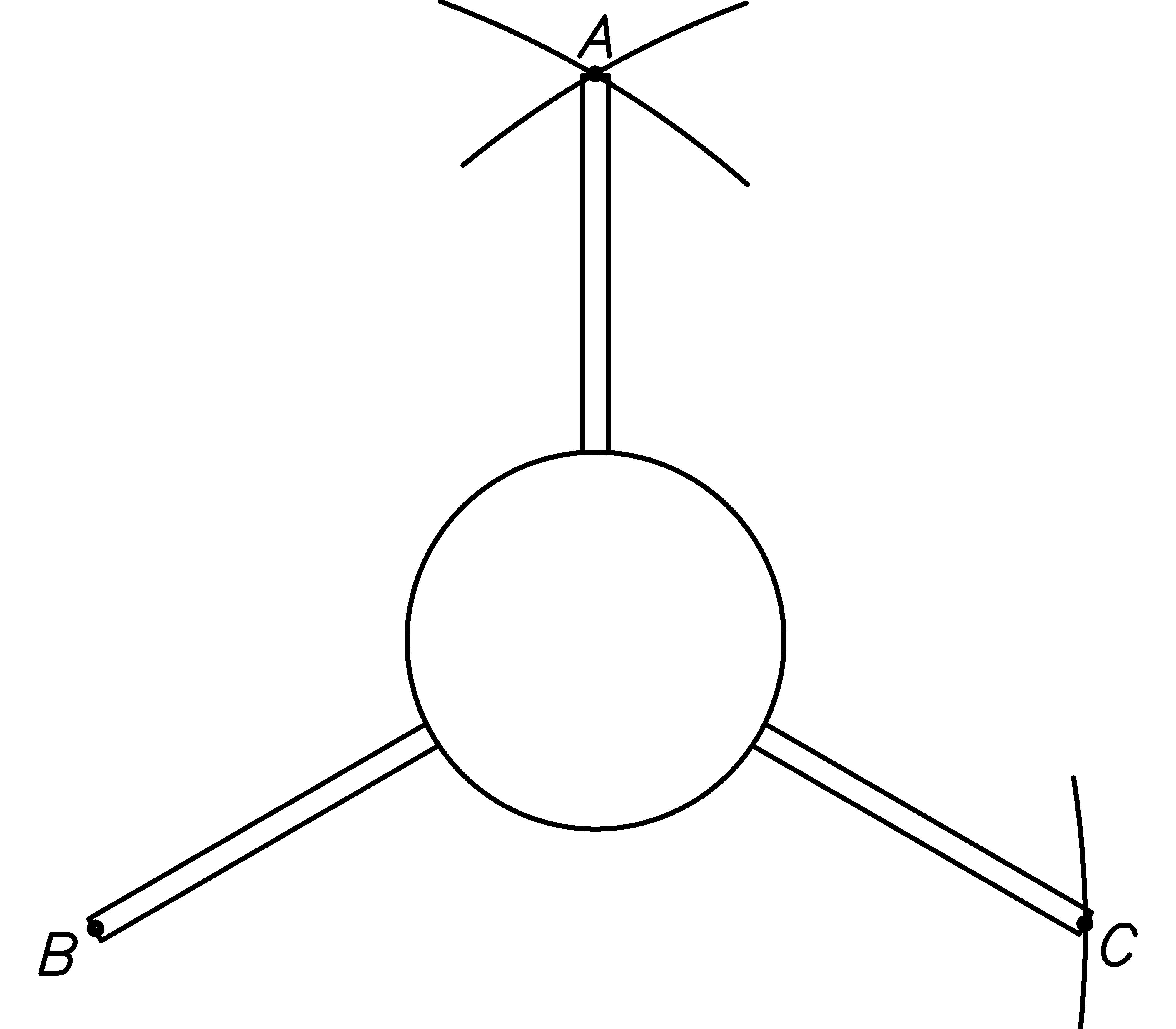
-
Measure the diameter of the circle passing through the 3 points: Find the center of the circle, then insert the compass anchor at the center and adjust so that the tip reaches the three points as closely as possible. Draw the circle, and measure the diameter with a ruler. [Hint: Euclid Book IV Proposition 5: Extend the perpendicular bisector of AB and AC until they intersect at circle’s center.]
4 Engine Thrust and Mass
Now that we’ve covered the basic calculations, drag, and spreadsheets, we are ready to fine tune our trajectory estimates even more. Using the spreadsheet you constructed for exercise 8↑ of the last chapter, let’s take a look at the difference 25 grams (about the mass of a C6-X engine), will make in the trajectory. Here are some of the output cell values:
|
Rocket Mass (g)
|
143
|
168
|
|
Apogee Height (m)
|
93.1199
|
75.9002
|
|
Apogee Time (s)
|
4.7600
|
4.5000
|
|
Maximum Velocity (m/s)
|
42.0846
|
35.3644
|
As the engines↓ get bigger (D, E, and beyond), their mass become a more significant factor in the trajectory. Also, remember that long before apogee, it is the mass of the fuel that has burned into gas and been left behind in Newton’s third law of motion↓↓↓ (action and reaction↓↓↓) that creating the rocket engine thrust.
At this point we need to understand how the fuel burns in more detail to come up with a better model of engine thrust and mass. Let’s take a look at a typical rocket engine in the figure below.‘
Notice the shallow hole in the bottom of the rocket engine. This is where the igniter is inserted and ignites the fuel (a substance similar to black powder or gun powder, only packed and bound into a cylindrical solid). The fuel starts burning at the ignition point and spreads from there in a uniform way.
The engine thrust results from the mass of the gasses produced (approximately equal to the mass of the fuel) accelerating out the bottom of the rocket engine (F = ma). The gasses are produced so fast that they push in all directions. The place with the least resistance is the bottom of the engine where the gas accelerates out. The shape of the exhaust hole (called a venturi↓) is important to the properties of the hot gas exhaust jet and thereby the functioning of the engine.
Newton’s law of equal action and reaction tells us that this accelerating matter (hot exhaust gas) is transformed into an equal force pushing the rocket engine in the opposite direction of the gas mass acceleration. Furthermore, we can now see that the force is in direct proportion to the amount of fuel burning, which is an expanding ball of fire.
Let’s assume the fuel burns in a homogeneous way (equal amounts and speeds in all directions) so that the resulting burn surface↓ (or burn front↓) is spherical in shape, at least at first. Furthermore, we’ll assume that the amount of force produced at a given time is proportional to the area of the burn surface. It turns out that the surface area of a sphere is proportional to the square of its radius (4πr2 to be precise), just as the perimeter of a circle is proportional to its radius (2πr).
We’ll take snapshots of the burn front as it progresses from ignition onward, with the snapshots equally spaced in time so that burn surface advances about one millimeter for each snapshot. Now, the inside diameter of a C6-X rocket engine casing is about 12 millimeters, so let’s take a look at how the surface area develops, measuring time in millimeters of burn, up until the burn front hits the cylinder walls. Note that 4π is approximately 12.566:
|
Time (mm)
|
Time^2 (mm^2)
|
Surface Area (mm^2)
|
|
0
|
0
|
0
|
|
1
|
1
|
12.6
|
|
2
|
4
|
50.3
|
|
3
|
9
|
113.1
|
|
4
|
16
|
201.1
|
|
5
|
25
|
314.2
|
|
6
|
36
|
452.4
|
At this point, the burning spherical surface starts to run out of fuel at the cylinder walls of the rocket engine casing, and decreases in size steadily, approaching a curved, disk-shaped plunger of fire moving up the inside of the rocket engine cylinder. From our diagram, we can guess that the time from hitting the cylinder walls until there is only a disk shaped plunger of fire will take about 2 or 3 snapshots. At this point, the 1/2 sphere surface area is about 226.2 square millimeters, but the area of a disk with a 6 millimeter radius is π62 or about 3.14⋅36 = 113.04 square millimeters. Let’s say the curved disk has a surface area that is the average of these two, about 170 square millimeters. Then we might reasonably fill in the rest of the table as follows:
|
Time (mm)
|
Surface Area (mm^2)
|
|
7
|
314
|
|
8
|
201
|
|
9
|
170
|
|
10
|
170
|
|
11
|
170
|
|
12
|
170
|
|
13
|
170
|
|
14
|
170
|
|
...
|
...
|
Let’s take a look at that graphically:
Recall the reasoning that the surface area of the burn is proportional to the engine thrust and suddenly you are looking at the rough shape (an estimate using our simplistic theoretical model) of the engine thrust profile↓↓! It isn’t nearly the constnat engine thrust profile we used in our trajectory calculations of the previous chapters. Furthermore, as the fuel burns, the engine mass decreases and further affects the trajectory calculations.
How can we incorporate all of this into improved trajectory estimates? At this point, there is no way around the use of a spreadsheet or computer program, and the best way for us to proceed is to use the spreadsheet constructed in exercise 8↑ of chapter 3↑. The general plan is as follows.
We’ll gather data for the engine of interest. Load it into our spreadsheet. Generate the derived values that we’ll need. Modify the Thrust column of the spreadsheet to use tabulated thrust data via interpolated table lookup. Modify the Acceleration without Drag and Drag columns of the spreadsheet to use adjusted mass (due to burned propellant). Finally, we’ll compare results from the more accurate engine model to results of the constant-thrust model.
Gather Engine Data
We start with actual engine thrust profiles↓ of the rocket engine of choice. Thanks to the National Association of Rocketry, the thrust profiles for many of the commercially available rocket engines are readily available on the internet at the following URLs:
-
http://www.nar/org/
-
http://www.thrustcurve.org/
-
http://www.modelrockets.us/thrustcurves.php
-
http://www.redarrowhobbies.com/
estes_model_rocket_engines.htm
For example, navigate your way on http://www.nar.org/ to the Rocket Motor Information link in the menu on the left margin of the page, then to the NAR Certified Motors link in the pop-up menu, then scroll down the table and click the C6 link for motors manufactured by Estes. This should bring up a PDF file in an appropriate viewer on your computer screen. The resemblance of the thrust profile plot to the burn front progression graph on page 4↑ gives us confidence in our theoretical model.
Advance to the second page of the document that lists the thrust profile as one pair of numbers per line. The first number is the time in seconds and the second is the thrust in Newtons. You’ll copy and paste these values into your spreadsheet in the next section.
If you are using a rocket engine for which you can’t find a detailed thrust profile, don’t despair. There are options, but they require more work. One possibility is to adapt the theoretical model we developed above to describe the engine you are using so that the resulting trajectory estimates are improved. The main problems will be knowing how to adapt the model and knowing how close to reality the model is. This brings us to a second option, which is, to measure the thrust profile yourself, under the supervision of a qualified person (check with a local middle or high school science teacher, they will probably want to set it up so that students can take part or observe).
Load Engine Thrust Data
We’ll assume the thrust profile↓ data for the engine, an Estes C6 engine in our example case, is displayed in a window on you computer and that you can copy it into your clipboard. Again, the data should be in a format that has the thrust profile as one pair of numbers per line, the first being the time in seconds and the second being the thrust in Newtons:
0.031 0.946
0.092 4.826
0.139 9.936
0.192 14.09
0.209 11.446
0.231 7.381
0.248 6.151
0.292 5.489
0.370 4.921
0.475 4.448
0.671 4.258
0.702 4.542
0.723 4.164
0.850 4.448
1.063 4.353
1.211 4.353
1.242 4.069
1.303 4.258
1.468 4.353
1.656 4.448
1.821 4.448
1.834 2.933
1.847 1.325
1.860 0.000
Now, open your trajectory estimate spreadsheet and notice the tabs↓ at the bottom of the page. Each tab corresponds to one spreadsheet. Usually there are three sheets↓ per file (named Sheet1, Sheet2, and Sheet3, but you can Insert, Append, or Remove sheets by right-clicking a tab and making the appropriate selection. Right-click on the trajectory estimate sheet tab and Rename it to Trajectory or something similar. Next right-click on the tab to the right and Rename it to something like EstesC6. Notice that this also makes the sheet active (brings it to the front so you can enter data).
Copy the data to the clipboard as follows. Make the window with the rocket engine thrust active. Select the thrust data (left-click in the upper left corner of the displayed numbers, drag down to the lower right corner while holding the click, then release). Copy it to the clipboard (select Edit, then Copy from the PDF viewer pull-down menu).
Finally, paste the data into the spreadsheet as follows. Make the spreadsheet window active. Position the cursor over the A9 cell, right-click, and select Paste. A Text Import Dialog box (or similar) should appear. Make the selections so that the data is deposited in the appropriate number of rows by two columns (in our Estes C6 case, cells A8:B31). Now go back up to cells A8:B8 and enter zero in each (this is missing in the data sets I’ve seen). Select the cell range A8:E39 and format for numeric values with three decimal places. Finally, enter Time values (to the next biggest tenth of a second, incrementing by a tenth of a second) for the remaining cells of the table so that we have values for the full table. Our use of the vlookup()↓ spreadsheet function will require Time values in every slot of the table, starting with zero and increasing as you move down the table.
|
Estes C6 Engine (from www.nar.org, except total mass)
|
|
8.817
|
Total Impulse (Ns)
|
|
10.800
|
Propellant Mass (g)
|
|
12.200
|
Remaining Mass w/o Delay (g)
|
|
1.833
|
Delay Mass (g)
|
|
|
|
|
|
|
|
|
Time(s)
|
Thrust(N)
|
Slope M
|
Intcpt B
|
Impls(Ns)
|
Used(Ns)
|
|
0.000
|
0.000
|
30.516
|
0.000
|
0.015
|
0.000
|
|
0.031
|
0.946
|
63.607
|
-1.026
|
0.176
|
0.015
|
|
0.092
|
4.826
|
108.723
|
-5.177
|
0.347
|
1.191
|
|
...
|
...
|
...
|
...
|
...
|
...
|
|
1.834
|
2.993
|
-123.692
|
229.785
|
0.028
|
8.781
|
|
1.847
|
1.325
|
-101.923
|
189.577
|
0.028
|
8.809
|
|
1.860
|
0.000
|
0.000
|
0.000
|
0.000
|
|
|
1.900
|
|
0.000
|
0.000
|
0.000
|
|
|
2.000
|
|
0.000
|
0.000
|
0.000
|
|
|
...
|
...
|
...
|
...
|
...
|
|
We’ll have a separate sheet for each of the different engines we want to model in the Trajectory spreadsheet, and look up the sheet by the name on the tab. It is important that we put the thrust data in the same place for each of the different engines sheets, so that when we look things up based on the engine name, we find the values we’re looking for in the same place on each sheet. Furthermore, the remaining spreadsheet structure should also be the same for each.
The Time and Thrust values together with some of the Engine Mass cells (discussed later) form the input cells of the rocket engine sheet, color their background accordingly. The remaining cells we’ll talk more about in the following sections.
Time (s) A8:A39. These values↓ (except for the first set of zeros and later Time values as described above) also come directly from the web page.
Thrust (N) B8:B39. These values↓ (except for the first set of zeros as described above) also come directly from the web page.
Generate Derived Values
The values derived↓↓↓ from the engine data fall into three categories: Thrust Profile, Engine Impulse, and Engine Mass. We’ll look at each of these in order.
Thrust Profile
In↓ order to take advantage of the thrust at each time increment of our trajectory calculations, we’ll need to find th thrust for each time increment. However, our time increments do not match the thrust data points we’ve gathered. To resolve this problem, we’ll take the approach of using a line segment to span the distance between two sample points. Then we’ll use the line to find values of thrust for times between two data points. Finding appropriate values between data points (especially in tabulated data) is known as interpolation↓↓, and since we are using a line to find the values between the points, it is known as linear interpolation↓↓↓.
Recall the equation of a line↓↓, y = Mx + B, from exercise 1↑ of chapter 1↑. For each pair of successive thrust measurement points, we’ll find the slope↓↓ M and intercept↓↓ B for the pairs of points and store these values in the spreadsheet alongside the 1st point of the pair.
For example, consider the successive thrust measurement points (0.031 s, 0.946 N) and (0.092 s, 4.826 N). First, let’s find the slope M as the proportion of thrust in Newtons to number of seconds for this time-section of the thrust curve. We’ll need to know not only an increment of time in seconds, but also the corresponding, equivalent increment of thrust in Newtons for this line segment section of the thrust curve:
From the diagram we can see that for this section of the curve, 3.880 Newtons is proportional to 0.061 seconds, so that we can find the slope M as the ratio 3.880 N ⁄ 0.061 s or approximately 63.607 N ⁄ s. M is a sort of conversion↓ from seconds to Newtons for this specific line segment. Before we move on to the intercept, let’s review this, rewriting it more symbolically, so we’ll know how to incorporate it into the spreadsheet more easily.
We started with two consecutive points (x1, y1) and (x2, y2). We then found the proportion of the change in vertical-axis values, y2 − y1, to the change in horizontal axis values, x2 − x1, and formed the slope of the line as the ratio M = (y2 − y1) ⁄ (x2 − x1) that converts horizontal units to vertical units.
To find the intercept B of the line, we’ll simply plug our first point (0.031 s, 0.946 N) and the approximate slope, 63.607 N ⁄ s, into the slope-intercept equation for a line, y = Mx + B, and solve for B to find an approximate value of -1.029:
0.946
=
63.607⋅0.031 + B
0.946
=
1.974607 + B
− 1.029
≈
B
Symbolically, we write this as: y1 = Mx1 + B or B = y1 − Mx1.
This gives us the formula for B in terms of M and the first point (x1, y1), and we are ready to incorporate this into the EstesC6 engine thrust sheet. Furthermore, we have already calculated some numeric values to check against. We’ll enter the formulas into the first row of the thrust table for the engine and then drag the formulas down the table. Notice in our symbolic expressions, that the y’s correspond to thrust, and the x’s correspond to time. Even though the following cells are outputs, I leave their backgrounds uncolored.
Slope (N/s) C8:C39. We’ll↓ translate our symbolic expression for slope described above into a formula using relative cell references and enter it into cell C8 as: =(B9-B8)/(A9-A8).
When you drag the formula down the table, check that the 2nd row entry is close to the approximate value we calculated above. Also, notice that the Slope cells toward the end of the table are zero, even though there are no corresponding Thrust values.
Intercept (N) D8:D39. We’ll↓ translate our symbolic expression for the intercept described above into a formula using relative cell references and enter it into cell D8 as: =B8-C8*A8.
Again, when you drag the formula down the table, check that the 2nd row entry is close to the approximate value we calculated above.
Engine Impulse
To↓ estimate the amount of fuel used (or remaining) at a given time, we’ll need to calculate the impulse inherent in the thrust profile data. To do this, we’ll calculate the impulse between pairs of thrust points and store the resulting impulse values in the Impulse column for the first point of each pair. Let’s look at this in more detail.
We’ll start, as before, with the following pair of successive thrust measurement points: (0.031 s, 0.946 N) and (0.092 s, 4.826 N). If the thrust were constant, say 0.946 Newtons for the whole time period, then we’d have an impulse of (0.092 s − 0.031 s)0.945 N = 0.057706 Ns for the time period. On the other hand, if the thrust were a constant 4.826 Newtons for the whole time period, we’d have an impulse of (0.092 s − 0.031 s)4.826 N = 0.294386 Ns for the time period. In each case, the value would just be the area under the curve.
For the non-constant thrust profile, we could break the time period into smaller and smaller sections, using an appropriate constant thrust value for each section. However, with each smaller subdivision we are approximating ever more closely the area under the thrust profile. This is the geometric reasoning that suggests we want the Newton-second area under the thrust profile curve for the impulse of the time period.
To find the impulse using our diagonal thrust profile line, we’ll want the area of the lower rectangle plus the area of the triangle having the diagonal as hypotenuse (half the area of the upper rectangle). We can find the impulse for this time period as:
(0.092 s
− 0.031 s)0.946 N + (0.092 s − 0.031 s)(4.826 N − 0.946 N) ⁄ 2
=
(0.092 s − 0.031 s)(4.826 N + 0.946 N) ⁄ 2
=
(0.061 s)(5.772 N) ⁄ 2
=
(0.061 s)(2.886 N)
=
0.176046 Ns
You may notice from either the geometry or the calculation, that this value is half way between the two extreme values we calculated above. It is their average. It is almost as easy to calculate as the extreme values. This sort of geometric and algebraic manageability is one of the things that makes linear models nice to work with. Now, let’s write it in more general symbolic notation using the points (x1, y1) and (x2, y2):
(x2 − x1)y1 + (x2 − x1)(y2 − y1) ⁄ 2 = (x2 − x1)(y2 + y1) ⁄ 2
That’s about as far as we can go symbolically, but it is far enough to help us generate impulse values for successive points in the thrust profile. We’ll translate this into a formula using relative references and store the result in the row of the first point. Even though they are all outputs, I only color the background of Total Impulse as an output cell.
Impulse (Ns) E8:E39. We’ll↓ translate our symbolic expression for impulse described above into a formula using relative cell references and enter it into cell E8 as: =(A9-A8)*(B9+B8)/2.
Check that the displayed value is similar to the numeric one we calculated above. When you drag the formula down the table, check that the Impulse cells toward the end of the table are zero when the corresponding Thrust value in that and the next row are both zero (or missing). Check that the displayed values are similar to the numeric values shown back on page 1↑.
Used Impulse (Ns) F8:F39. When↓ we incorporate engine mass into the spreadsheet, we’ll need the accumulated impulse used up to the time of the Thrust Profile table row. In order to form this value, we sum the values in previous rows of the table. (We insist that the Impulse value in the row of labels, cell E7, be zero to simplify the formula.) We can then enter the following formula into cell F8 as: =sum($E$7:E7).
Notice that the first cell reference is absolute, staying constant as we drag the formula down the table, but the second cell reference is relative, changing the range to include all previous rows as we drag.
Total Impulse (Ns) A2. We’ll↓ need to accumulate all of the impulse values into the total impulse. We’ll add them all up by entering the following formula in cell A2: =sum(E8:E39).
Engine Mass
We’ll↓ use a simple model of engine mass that consists of only two parts: the propellant mass, and the mass of the remaining (non-propellant) part of the engine. The propellant mass is entered directly from the web page. The remaining mass is complicated by the fact that there is a significant difference in mass depending on whether or not an engine has a delay (zero-second delay engines are a few grams less). Also complicating the remaining mass portion are the slight variations with differing delays and rocket engine manufacturing batches (which probably also effect propellant mass).
To deal with the added complication of variation in remaining mass, we’ll construct a table and average some data. The table will consist of two columns, one for the delay in seconds, another for the total engine mass. The first few rows of the table contain values for zero-second delay engines (followed by their average), and the remaining rows of the table contain values for engine with delays (again, followed by their average). For example:
|
Estes C6 Engine (from www.nar.org, except total mass)
|
|
8.817
|
Total Impulse (Ns)
|
Delay(s)
|
Eng Mass(g)
|
|
10.800
|
Propellant Mass (g)
|
0
|
23
|
|
12.200
|
Remaining Mass w/o Delay (g)
|
0
|
23
|
|
1.833
|
Delay Mass (g)
|
Average(g)
|
23.000
|
|
|
|
3
|
24
|
|
|
|
3
|
25
|
|
|
|
3
|
25
|
|
|
|
5
|
25
|
|
|
|
5
|
25
|
|
|
|
5
|
25
|
|
|
|
Average(g)
|
24.833
|
The web page contains values you can use in the table. However, measuring your own values will probably reflect the reality of your circumstances more accurately, especially if you use the engines you measure. In this spirit, I’ve listed values for some of the engines I’ve measured (but, feel free to use the masses listed on the web page instead if you choose to). The first three categories below are input cells, the next two are derived, and the last two are output cells.
Propellant Mass (g) A3. This value↓ comes directly from the rocket engine web page.
Engine Delay (s) G3:G4, G6:G11. These delay values↓ are from the engines I measured.
Engine Mass (g) H3:H4, H6:H11. These are the mass↓ values I measured for the engines I had on hand.
Average Engine Mass w/o Delay (g) H5. The average mass↓ of engines having a zero-second delay: =average(H3:H4).
Average Engine Mass w/Delay (g) H12. The average mass↓ of engines having a non-zero delay: =average(H6:H11).
Remaining Mass w/o Delay (g) A4. The average mass↓ of engines having a zero-second delay minus the mass of the propellant: =H5-A3.
Delay Mass (g) A5. The average mass↓ of engines having a non-zero delay minus the average mass of engines having a zero-second delay: =H12-H5.
Incorporate Improved Thrust
We are now ready to incorporate our improved rocket engine thrust model into the Trajectory Calculations table. The main idea will be to use the current time value to look up the appropriate slope and intercept values from the rocket engine thrust table, then plug the time value into the slope-intercept line equation to calculate the corresponding thrust and use that value. This is pretty complicated compared to our previous spreadsheet work, so we’ll take it step at a time.
We’ll use the current time value as one of the parameters in the vlookup()↓ spreadsheet function to look up the appropriate slope and intercept values for the line segment of the thrust profile. However, unlike when we used the function in chapter 3↑ to look up the Mass using the Rocket name, here there are a few complications that require some explanation.
First, since we’ll look the current time up in a table where we cannot expect the exact value will be found, we cannot use an exact value lookup. We’ll have to use an approximate lookup. This requires that the table be organized with time values in increasing order. Luckily, the thrust profile data already complies with this requirement. Furthermore, in case vlookup() cannot find an exact match, it will return as an approximate match the largest value that is less than the one sought. This is why we stored the slope and intercept values alongside the first (lesser time value) of the thrust data points.
Another difference is that we are looking up values from a different sheet. To do this, we have to include the sheet name as a prefix in the cell range specification. For example, to specify the Thrust Profile table in the EstesC6 sheet we’ll use the expression EstesC6!$A$8:$F$39. With this in mind, and assuming the current time is in cell A28, we can look up the approximate Slope entry of the Thrust Profile table using the following parameters for vlookup():
-
The value to match. We want the input to come from A28. However, since we might drag this formula over to another column for debugging, but still want the value from column A we’ll use an absolute reference for the column. On the other hand, when we drag the formula down, we want the row number of increment, so we’ll use a relative reference for the row. Thus the reference will be: $A28.
-
Range of table cells. As mentioned above, we’ll specify the fixed-location Thrust Profile table using absolute references as: EstesC6!$A$8:$F$39.
-
Column to select. The table value we want is the Slope, in the third column of the table, column C, so we use the value: 3.
-
Approximate? As explained above, we want approximate lookup, so we use the value 1.
-
Return index? This optional true-or-false (boolean) parameter defaults to false, which is just what we want. We won’t even list the value so that we can export the spreadsheet in Excel format if we want.
Putting this all together, we come up with the following expression for the Slope from the Thrust Profile table for the current time:
vlookup($A28,EstesC6!$A$8:$F$39,3,1)
Similarly, we have the the following expression for the Intercept from the Thrust Profile table for the current time:
vlookup($A28,EstesC6!$A$8:$F$39,4,1)
It is now easy to use the slope-intercept formula for a line to construct the thrust for the current time as the expression:
$A28*vlookup($A28,EstesC6!$A$8:$F$39,3,1)+
vlookup($A28,EstesC6!$A$8:$F$39,4,1).
The last complication arises from the fact that rather than coding the engine sheet name into the formulas of the Trajectory Calculations table, we’d rather reference cell A12 that contains the Engine name. That way, in order to use a different engine in the trajectory calculations, we need only change one cell of the spreadsheet. To do this, we’ll need to construct the cell range expressions using the indirect()↓ and concatenate()↓ spreadsheet functions. We’ll splice the Engine name to the Thrust Profile table range string in the expression concatenate($A$12,”!$A$8:$F$39”).
However, just replacing the reference EstesC6!$A$12:$F$39 with this expression won’t work. That’s because the spreadsheet thinks the result of the concatenate() function is a string, not a cell reference. In order to specify the cell reference (and get the value), we have to run it through the indirect() function as:
indirect(concatenate($A$12,”!$A$8:$F$39”))
Finally, in this way, we arrive at the formula we enter into cell B28 as the Thrust for the current Time (A28) in the Trajectory Calculations table as:
$A28*vlookup($A28,
indirect(concatenate($A$12,”!$A$8:$F$39”)),3,1)+
vlookup($A28,
indirect(concatenate($A$12,”!$A$8:$F$39”)),4,1).
Once you have the new thrust formula entered (altogether on one line), verify that the numeric value is zero. This is due to the rocket engine starting its burn with zero Newtons of thrust. Next, drag the formula down the B column of the Trajectory Calculations table and verify the thrust values agree with the thrust profile.
You may also notice a resulting oddity in the velocity column. The rocket starts moving down! It’s as if we were holding the rocket off the ground at the time of launch, and dropped it at engine ignition. We have not included the constraint that the rocket is initially being supported by the ground. It supplies the force required to keep the rocket from falling.
We’ll resolve this difficulty by adjusting the formulas in the velocity column as follows. We’ll only add in the velocity increment generated from the acceleration when either the acceleration (E28) or the height of the rocket (G28) is greater than zero. We’ve talked about the spreadsheet if()↓ function before, but we’ll also need the spreadsheet or()↓ function. The resulting formula we’ll enter into cell F29 is: if(or(E28>0,G28>0),E28*$F$13+F28,0).
Incorporate Improved Engine Mass
We are now ready to incorporate our improved rocket engine mass model into the Trajectory Calculations table, however, this is even more complicated than the improved thrust model. Let’s begin with the easier modifications and save the complications for last. The first order of business is to add an input cell to the Flight Combination to specify the number of seconds of delay for the Rocket Engine, followed closely by the addition of a new derived input Engine Burn to the Trajectory Constants. Then we’ll convert Total Impulse and Average Thrust inputs to derived cells, and modify the Rocket Mass. We’ll also add the Coast time output cell to the Trajectory Estimates section before we move on.
Rocket Engine Delay (s) B12. Simply type this value↓ into the cell. The main distinction is whether or not the value is zero. Non-zero delays have increased engine mass. Zero delay engines are only for the first stage of multistage rockets (see exercise 8↑ of chapter 3↑). For example, enter the value 3.
Engine Burn (s) I14. We’ll glean the length of the engine burn↓ as the time of the first zero Thrust entry in the Trajectory Calculations table (not counting Time 0) and use it to calculate the average thrust and coast times. Just as before (Apogee(s) page 6↑) we’ll use the match()↓ and index()↓ spreadsheet functions: =index($A$29:$A$1028,match(0,$D$29:$D$1028,0)).
Total Impulse (Ns) F14. We convert this input cell to a derived value↓ that is now available from the rocket engine sheet specified by the Flight Combination via:
indirect(concatenate($A$12,”!$A$2”)).
Average Thrust (N) F15. We convert this input cell to a derived value↓ as the fraction Total Impulse divided by Engine Burn: =$F$14/$I$14.
Rocket+Engine Mass (N) A22. First, we update the label, then the value as well. For the value, we must add in the rocket engine mass. The trick is that if there is a non-zero delay, we need all three cells A3:A5 from the rocket engine sheet, but only A3:A4 for a zero delay engine. We take care of this with the if() function when forming the cell range reference:
=(vlookup($A$11,$A$6:$J$8,3,0)+
sum(indirect(concatenate($A$12,
if($B$12>0,"!$A$3:$A$5","!$A$3:$A$4")))))/1000.
Coast Time (s) I23. With the addition of Engine Burn, this output cell value↓ is easy to calculate as: =$F$23-$I$14.
Things get a bit stickier for these last few modifications to the Trajectory Calculations↓ table. What we’ll be doing is to add a couple of columns to the table, one to keep track of how much of the fuel is used at the current time, and the other to reflect the corresponding mass of the rocket. First, make space for the new rows by selecting the cell range B26:G1028, cutting it, and pasting it over on the right side, at cell H26. Now, while it is still selected, right-click inside it at cell H26 and cut it again, and then paste it into cell D26. Then arrange the labels so that the top-left portion of the table looks something like this:
|
Time
|
Fuel Used
|
Mass
|
Thrust
|
w/o Drag
|
Drag
|
w/Drag
|
...
|
|
(s)
|
(frac)
|
(kg)
|
(N)
|
Acc(m/ss)
|
(m/ss)
|
Acc(m/ss)
|
...
|
|
0.000
|
|
|
6.000
|
32.1514
|
0.0000
|
32.1514
|
...
|
|
0.010
|
|
|
6.000
|
32.1514
|
0.0000
|
32.1514
|
...
|
|
0.020
|
|
|
6.000
|
32.1514
|
-0.0007
|
32.1507
|
...
|
|
0.030
|
|
|
6.000
|
32.1514
|
-0.0027
|
32.1486
|
...
|
|
...
|
...
|
...
|
...
|
...
|
...
|
...
|
...
|
|
4.780
|
|
|
0.000
|
-9.8066
|
0.0002
|
-9.8058
|
...
|
|
4.790
|
|
|
0.000
|
-9.8066
|
0.0005
|
-9.8053
|
...
|
|
...
|
...
|
...
|
...
|
...
|
...
|
...
|
...
|
Fuel Used (frac) B28:B1028. These values↓ range from 0 at ignition, to 1 at the time the engine cuts out. The idea is to form a current used impulse and divide by the Total Impulse. We’ll lookup Used Impulse in the Thrust Profile table and add in the incremental impulse for the current time. We’ll form the incremental impulse from Thrust (looked up in the Thrust Profile table) and the current Thrust. Recall that the impulse will be given by (x2 − x1)(y2 + y1) ⁄ 2. Notice that the current time x2 is in cell A28, the current thrust y2 is now in cell D28, and the total impulse is in cell F14. With this in mind, we can formulate the fuel used fraction for the EstesC6 engine into cell B28 as:
=(vlookup($A28,EstesC6!$A$8:$F$39,6,1,0)+
0.5*($D28+vlookup($A28,EstesC6!$A$8:$F$39,2,1))*
($A28-vlookup($A28,EstesC6!$A$8:$F$39,1,1))/$F$14.
To generalize this for the engine in $A$12, substitute the expression: indirect(concatenate($A$12,"!$A$8:$F$39")) for each cell range: EstesC6!$A$8:$F$39 above.
Upon entering the formula, you should see the value 0 appear. When you drag it down the column, the values should increase steadily to the value 1 at engine cut-out and then remain 1 to the end of the table.
Mass (g) C28:C1028↓. In C28 we’ll convert Propellant Mass to kilograms, scale it by the Fuel Used fraction and subtract it from Rocket+Engine Mass to get time varying rocket mass:
=$A$22-$B28*indirect(concatenate($A$12,"!$A$3"))/1000.
Upon entering the formula, you should see the the full Rocket + Engine Mass value appear. When you drag it down the column, the values should decrease steadily to reflect the loss of all propellant mass at engine cut-out and then remain there to the end of the table.
Acceleration without Drag (m/ss) Now E28:E1028. Edit↓ the formula =B28/$A$22-$F$12 in cell E28 and replace any cell reference $A$22 to static, pre-flight rocket mass with $C28 for the current, time-varying mass: =B28/$C28-$F$12. Drag the formula down the table, and scroll through the spreadsheet to verify the numbers.
Drag (m/ss) Now F28:F1028. Edit↓ our previous formula in cell E28: =-sign(F28)*$F$11*$A$23*$A$24*F28*F28/(2*$A$22) replacing any cell reference $A$22 to static, pre-flight rocket mass with $C28 for the current, time-varying mass:
=-sign(F28)*$F$11*$A$23*$A$24*F28*F28/(2*$C28).
Drag the formula down the table, and scroll through the spreadsheet to verify the numbers.
Comparison
I’ll list the resulting trajectory estimates that include the improvements in this chapter here so you can use the values to compare against you own spreadsheet:
|
Time
|
Used
|
Mass
|
Thrst
|
Acc no
|
Drag
|
Acc w
|
Vel
|
Ht
|
|
(s)
|
(frac)
|
(kg)
|
(N)
|
Drag
|
(m/ss)
|
Drag
|
(m/s)
|
(m)
|
|
0.000
|
0.000
|
0.16783
|
0.000
|
-9.8066
|
0.0000
|
-9.8066
|
0.0000
|
0.0000
|
|
0.010
|
0.000
|
0.16783
|
0.305
|
-7.9884
|
0.0000
|
-7.9884
|
0.0000
|
0.0000
|
|
0.020
|
0.001
|
0.16783
|
0.610
|
-6.1700
|
0.0000
|
-6.1700
|
0.0000
|
0.0000
|
|
0.030
|
0.002
|
0.16782
|
0.915
|
-4.3514
|
0.0000
|
-4.3514
|
0.0000
|
0.0000
|
|
0.040
|
0.003
|
0.16780
|
1.518
|
-0.7575
|
0.0000
|
-0.7575
|
0.0000
|
0.0000
|
|
0.050
|
0.005
|
0.16778
|
2.155
|
3.0348
|
0.0000
|
3.0348
|
0.0000
|
0.0000
|
|
0.060
|
0.008
|
0.16775
|
2.791
|
6.8289
|
0.0000
|
6.8289
|
0.0303
|
0.0000
|
|
0.070
|
0.011
|
0.16771
|
3.427
|
10.6253
|
0.0000
|
10.6253
|
0.0986
|
0.0003
|
|
0.080
|
0.016
|
0.16767
|
4.063
|
14.4245
|
-0.0001
|
14.4245
|
0.2049
|
0.0013
|
|
...
|
...
|
...
|
...
|
...
|
...
|
...
|
|
...
|
|
1.820
|
0.990
|
0.15714
|
4.448
|
18.4490
|
-6.0131
|
12.4859
|
31.6572
|
33.1295
|
|
1.830
|
0.994
|
0.15709
|
3.399
|
11.8312
|
-6.0631
|
5.7681
|
31.7820
|
33.4461
|
|
1.840
|
0.998
|
0.15706
|
2.292
|
4.1425
|
-6.1129
|
-1.9703
|
31.8397
|
33.7639
|
|
1.850
|
0.999
|
0.15704
|
1.019
|
-3.3164
|
-6.1364
|
-9.4528
|
31.8200
|
33.0823
|
|
1.860
|
1.000
|
0.15703
|
0.000
|
-9.8066
|
-6.1296
|
-15.9362
|
31.7255
|
34.4005
|
|
...
|
...
|
...
|
...
|
...
|
...
|
...
|
...
|
...
|
|
4.580
|
1.000
|
0.15703
|
0.000
|
-9.8066
|
-0.0003
|
-9.8069
|
0.1213
|
74.3240
|
|
4.590
|
1.000
|
0.15703
|
0.000
|
-9.8066
|
-0.0001
|
-9.8067
|
0.0232
|
74.3252
|
|
4.600
|
1.000
|
0.15703
|
0.000
|
-9.8066
|
0.0000
|
-9.8067
|
-0.0749
|
74.3255
|
|
4.610
|
1.000
|
0.15703
|
0.000
|
-9.8066
|
0.0000
|
-9.8066
|
-0.1730
|
74.3247
|
|
4.620
|
1.000
|
0.15703
|
0.000
|
-9.8066
|
0.0002
|
-9.8065
|
-0.2710
|
74.3230
|
|
...
|
...
|
...
|
...
|
...
|
...
|
...
|
...
|
...
|
Let’s compare estimate outputs for the case of the simplistic engine model, the improved engine model, and a hybrid model that is the simplistic model that includes the mass of the engine with half of the propellant and total impulse equal to the improved model:
|
|
Simple
|
Improved
|
Hybrid
|
|
Apogee (m)
|
92.3015
|
74.3255
|
76.3255
|
|
Apogee (s)
|
4.7400
|
4.6000
|
4.4800
|
|
Maximum Velocity (m/s)
|
41.8786
|
31.8397
|
35.9668
|
|
Coast Time (s)
|
3.2400
|
2.7400
|
3.0100
|
We can see that the decreased mass and extra total impulse is a significant difference between the simple and improved models. Beyond that, the time varying nature of the thrust and mass is still a significant difference between the improved and hybrid model. Even though the hybrid and improved outputs are within 15% of each other, the largest difference is in the maximum velocity and effects the very motion that we are trying to estimate.
Exercises
-
Modify the spreadsheet you created in exercise 8↑ of chapter 3↑ to:
-
Create an engine data sheet for an Estes C6 engine.
-
Incorporate the refinements described in this chapter for engine thrust for the C6 engine.
-
Incorporate the refinements described in this chapter for the engine mass for the C6 engine.
-
Use the spreadsheet from exercise 15↑ above to generate multistage↓ trajectory estimates (take a look exercise 8↑ of chapter 3↑ for further details on multistage rockets and RedDevil rocket properties).
-
Create an engine data sheet for an Estes D12-0 engine.
-
Don’t forget to add the mass of the second stage C6-3 rocket engine when constructing the Rocket Properties table row for the RedDevil.
-
For the RedDevil, EstesD12 Flight Combination, find the time, velocity, and height at the time the D12 engine cuts out.
-
For the RedPhoenix, EstesC6 Flight Combination, enter the initial velocity and height you collected in part (b) above, and record the apogee height, maximum velocity, and flight time (as the sum of the apogee time of the second stage and the time until engine cut off collected in part (a)) for the two stage rocket flight.
-
If you did exercise 8↑ of chapter 3↑, compare the results.
5 How High Did It Go?
Once we have our rocket, weighed it, measured it, and plugged in all the parameters to get our best estimate of the trajectory, we can select the engine delay and actually load and launch the rocket. However, a big piece of the estimation process (perhaps the most important piece), is comparing the estimates to actual results.
So, how do we measure how high the rocket goes on its actual flight? There are two common ways. One is to insert an altimeter into the payload bay of your rocket (be sure to include the mass in the trajectory calculations) and have it collect data for the flight. This is the preferred option, since you get height readings at regular intervals. After the flight, the data is available for download to a computer with software that comes with the altimeter. However, for simple rockets without a payload bay, or in case you don’t care to spend hard-earned money on this sort of thing, there is another, geometric way of determining how high the rocket went.
The geometric method was used by ancient Greeks to determine how far a ship was out to sea. The main idea is based on the proposition that the lengths of sides of similar triangles are in common proportion. In the diagram below, we can’t measure the large triangle, but we can measure a similar, smaller one. In fact, if we use some modern mathematics, we don’t even need to measure the smaller one.
I’ll describe a primitive, low tech method, but we’ll need the following:
-
An approximately vertical rocket flight.
-
An approximately level and flat launch area.
-
To be able to see the rocket at apogee.
-
A couple of meter sticks to measure distance on the ground.
-
A sightable angle measuring device (made from a couple of sticks and a bolt).
-
Some geometry and geometric tools (compass, ruler, protractor).
The idea is to measure both our distance from the launchpad, and the viewed angle from launchpad height to apogee height. Next we’ll need a smaller, more manageable, similar triangle so that we can get its base and height lengths. Finally we calculate the apogee using the proportionality of the similar triangles.
Measure Distance and Angle
You can use a couple of meter sticks to measure off a distance from the launchpad by laying one stick down in front of the other as you move away from the launchpad. It works even better if you have, say, 4 or 5 meter sticks and a friend to help. The most accuracy results from an angle near 450, so it is better to measure out a distance near the expected apogee.
To measure the angle of the rocket at apogee, you need an angle measuring device. You can make one from a couple of flat pieces of wood such thin meter or yard sticks. Just drill holes at one end of each stick, about in the center of the stick. For instance if the stick is 1 inch wide, drill a hole about 1/2 inch in from the end and each of the sides, just large enough for a screw and nut. Put the screw through the holes and tighten the sticks together with a lock-nut, tight enough to maintain the angle of separation when the sticks are released, but not so tight that the sticks cannot be easily separated.
To use the device at the time of launch, close the sticks together and sight along them, level to the ground, toward the rocket on the launchpad. As the rocket rises, with one hand keep one of the sticks level to the ground and pointing to where the rocket was, and with the other hand raise the other stick so that you sight the rocket along it as it rises to apogee. All the while, you have the corner of the device (where the two sticks are bolted together) stuck in your face, almost touching your eye. All this manipulation may take some practice to master, so try it a few times before you launch the rocket.
Once you have captured the angle accurately, measure it with the protractor as accurately as possible. The accuracy with which you measure this angle will probably be the determining factor of the accuracy of the resulting apogee value.
Smaller Similar Triangle
One possibility for reproducing the launchpad-apogee-viewing triangle is to create it on a piece of paper. A horizontal line will represent the line from viewer to launchpad. A vertical line (at 90 to the horizontal) will represent the line from apogee to launchpad. Either use graph paper for the horizontal and vertical lines, or draw them yourself, being sure to construct the lines at 90 degrees as carefully as possible. From the 90 degree angle (this represents the launchpad) measure out a convenient distance, say 20 centimeters, and mark a point on the horizontal line (this represents the viewpoint). Finally, as precisely as possible, reproduce the measured angle at the viewpoint (either by tracing the measuring device or with a protractor), and continue the angled line until it intersects the vertical line. Now measure the height to where the vertical and angled lines intersect. Let’s denote this measured height by h and the 20 centimeters (or whatever) distance of the base with b.
If you are willing to invest in a little bit of advanced mathematics, we can do much better than this crude triangle construction and measuring business with a calculator or computer. In the years since the ancient Greeks, mathematicians have made a study of the measurement of angles and triangles. It is more commonly known as trigonometry↓ and a large part of it focuses on right triangles that fit in a unit circle, with the hypotenuse being a radius of the circle.
The angle α is measured counterclockwise from the positive x-axis, and as the angle progresses from 00 to 900, the base of the triangle goes from 1 to zero on the x-axis, and the height of the triangle goes from 0 to 1 on the y-axis. Then as the angle continues from 900 to 1800, the base goes from 0 to -1 on the x-axis, and the height goes from 1 to 0 on the y-axis. As the angle grows, the height continues on into the negative y-values to -1, then increases again toward +1. You can also imagine the angle growing in the negative, clockwise direction.
The function that converts the angle α into the y-axis value is known as the sine↓↓ function, abbreviated sin, and we write the sine of the angle α as sin(α), though many write it as just sin α. Similarly, the corresponding function (co-function) that converts the angle α into the x-axis value is known as the cosine↓↓ function, abbreviated cos, and we write the cosine of the angle α as cos(α), though many write it as just cos α. There are many interesting and surprising relationships to be explored in and between these functions and angles, including a magical formula that lets us calculate the sine and cosine function values to any precision we like. Much of this forms the basis for a course in trigonometry and/or calculus. However, for our purposes, we’ll just use a handy calculator, computer, or even (egads!) a cell phone to calculate the sine and cosine of our measured angle. Just as above, we’ll call the sine value h, and the cosine value b (for height and base respectively). Be sure that you have the calculator (computer, or whatever) in the mode where inputs tor these functions are specified in degrees (not radians). You can check this by entering the value 45 and getting back answers approximating the square root of 2 divided by 2, approximately 0.70710678.
Calculate the Apogee
Now that we have the measured distance from the viewpoint to the launchpad, lets call it B, and the lengths of h, and b for the smaller, similar triangle, we can solve for the apogee, call it H, as follows. We simply setup an equation that expresses the equality of the common proportion (or scale factor) between the similar triangles:
Now multiply both sides by h to solve for H:
For example, suppose we have the following values: h = 0.8, b = 0.6, and B = 100 m. Then we find that the apogee is approximately 133.3 meters.
Exercises
-
Suppose that you measure off 100 meters for B and have limited the measured angle to apogee to definitely lie between 66 and 67 degrees. What is the corresponding range in apogee?
-
Use the Pythagorean Theorem (equation for the squares of the lengths of the sides of a right triangle) and a square of side x and diagonal 1 to show that both the sine and cosine of a 45 degree angle is exactly the square root of 2 divided by 2.
6 Further Investigations
Here is a collection of ideas that come to mind. Hopefully, they will sound interesting to you, or, perhaps, spark some of your own new ideas for further investigation. In any case here they are:
-
Rather than use a spreadsheet, write a program that generates trajectory estimates. Extend the program so that you can also input actual flight trajectory data (from an altimeter) and compare it to estimates. Extend the program even further to adjust parameters that make the estimates closer to the actual data. This takes you into the field of optimization, and if you intend to give it a try you might want to start by finding a text that has a friendly introduction at a level that suits your interests and background.
-
Investigate air density as an ideal gas taking into consideration humidity, temperature, and altitude. One place to start is the http://www.en.wikipedia.org/wiki/Density_of_air. However, it might be more understandable and enjoyable to use the more leisurely approach of a text like An Introduction to Thermal Physics by C. J. Adkins.
-
Come up with an analytic model for the coefficient of drag, by using the drag surface area of in combination with the angle of inclination the various patches of drag surface. A further extension might think of the flow of air around the rocket in layers like nested balloons, where the natural state (without the rocket) is like a long thin empty balloon, but that as the rocket passes through, the balloon must be blown up to the shape of the rocket. Think of the balloon pressing on the sides of the rocket, causing friction. The more you blow up the balloon and separate its sides, the more friction on the rocket there would be, with the primary source of friction being the drag surface.
-
Design, setup, and use a wind tunnel to test the various surface sizes, shapes, and materials, and test various drag coefficient analytic models and values.
-
Investigate the various NAR allowed engine fuels and compare the impact of the various mass, burn, and thrust characteristics on trajectory estimations. Extend this to include different initial packing and ignition geometries on thrust profiles and resulting trajectories.
-
Design setup, and use an engine thrust measurement system to test various engines. Vary the engine sizes, fuels, geometries.
-
Refine the engine mass model to include the slow burning of delay mass.
-
Develop a theoretical ground model and investigate the impact crater of an object by incorporating it into the trajectory calculations. Model the ground with various densities and viscosities and compare the impact craters.
-
Investigate the effect of a model improvement (engine mass, fuel composition, air density, drag coefficient, ...) across different flight combinations (rocket mass, engines of differing total impulse and average thrust).
-
Investigate the sensitivity of trajectory estimation across various parameters (mass, fuel, total impulse, average thrust, drag coefficient, air density, ...).
7 Resources
Once you start looking, you may be surprised to find how much information on Model Rocketry there is online. Here are some links to get you started:
-
http://en.wikipedia.org/wiki/Model_rocket
-
http://exploration.grc.nasa.gov/education/rocket/rktengperf.html
-
http://www.modelrockets.us/index.php
-
http://www.nar.org/
-
http://www.tripoli.org/
-
http://www.rocketsnw.com/
-
http://www.grc.nasa.gov/WWW/K-12/airplane/rockth.html
-
http://www.apogeerockets.com/education/index.asp
For those of you who are not adverse to looking through more advance mathematics, let me point out a few links that got me started with my trajectory estimates:
-
http://www.apogeerockets.com/education/
downloads/numeric_methods.pdf
-
http://www.esteseducator.com/Pdf_files/Part_1.pdf (also parts 2,3,... though I haven’t been able to get through to this website for a while now)
A marvelous rocket simulator call OpenRocket is freely available. It is based on the Masters thesis by Sampo Niskanen you can find more at:
-
http://openrocket.sourceforge.net/
Furthermore, you’ll probably turn up even more about model rocketry by searching for the following (or your own more specific) key words:
-
Model Rocketry
-
Model Rockets
-
Rocket Engines
-
Rocket Aerodynamics
In addition, the following books are fantastic sources for more information and further reading:
G. Harry Stine, Bill Stine: Handbook of Model Rocketry, Seventh Edition. A great general purpose resource for all aspects of Model Rocketry.
David Berlinski: Newton’s Gift: How Sir Isaac Newton Unlocked the System of the world. A celebration of the system of thought that created physics, and the man who gave it to us.
Index
:
MKS system:
acceleration units: ↑
force equation: ↑
velocity units: ↑
MKS system: ↑
Newton:
first law of motion: ↑
force law: ↑
law of action and reaction: ↑
law of inertia: ↑
second law of motion: ↑
third law of motion: ↑
units of force: ↑
acceleration:
gravitational: ↑, ↑, ↑
measurement: ↑
units: ↑
vector: ↑
acceleration: ↑
accumulate: ↑
air:
density: ↑, ↑, ↑
resistance: ↑
viscosity: ↑
apogee:
apogee: ↑
burn front: ↑
burn surface: ↑
cell:
comment: ↑
derived input: ↑
derived input: ↑
formatting: ↑
input: ↑
input: ↑
numeric: ↑
output: ↑
range:
range: ↑
reference:
absolute: ↑, ↑, ↑
absolute: ↑
circular: ↑
relative: ↑, ↑
relative: ↑
reference: ↑
trajectory calculation: ↑
cell: ↑
coast:
code walk-through: ↑
coefficient: ↑
conversion factor: ↑
conversion factors: ↑, ↑, ↑
cosine: ↑, ↑
debugging:
code walk-through: ↑
error identification: ↑
expected output: ↑
test case: ↑
debugging: ↑
density:
air: ↑, ↑
measurement: ↑
units: ↑
density: ↑
derived inputs:
drag area: ↑, ↑
drag coefficient: ↑
drag surface area: ↑
rocket mass: ↑
spreadsheet cells: ↑
dimension analysis: ↑
discrete sampling: ↑
drag:
coefficient: ↑
coefficient: ↑
fins: ↑
nose cone: ↑
properties: ↑
surface area: ↑, ↑, ↑, ↑, ↑
surface area: ↑
term: ↑
drag: ↑
engine impulse:
impulse: ↑
total impulse: ↑
engine mass:
average engine mass w/delay: ↑
average engine mass w/o delay: ↑
delay mass: ↑
delay: ↑
engine mass: ↑
propellant mass: ↑
remaining mass w/o delay: ↑
engine|seerocket engine: ↑
equation:
line: ↑
line: ↑
parabola: ↑
error identification: ↑
expected output: ↑
flight combination:
engine: ↑
rocket engine delay: ↑
rocket: ↑
force:
equation: ↑
equation refined: ↑
equation with drag: ↑
equation: ↑
gravity: ↑, ↑
measurement: ↑, ↑
rocket engine: ↑
thrust: ↑
units: ↑
vector: ↑, ↑
force: ↑
formatting spreadsheet cells: ↑
formula:
dragging: ↑
example: ↑
geometric: ↑
formula: ↑
function:
cosine: ↑, ↑
linear: ↑
quadratic: ↑
gravity: ↑
acceleration: ↑, ↑, ↑
force: ↑, ↑
weight: ↑
impulse: ↑, ↑
inertia: ↑
inertia: ↑
initial conditions:
initial conditions: ↑
inputs:
derived: ↑, ↑
derived: ↑
spreadsheet cells: ↑
spreadsheet cells: ↑
intercept: ↑
interpolation:
interpolation: ↑
kinetic energy: ↑
law:
first law of motion: ↑
of action and reaction: ↑
of force: ↑
of inertia: ↑
second law of motion: ↑
third law of motion: ↑
line:
equation: ↑
intercept: ↑
interpolating: ↑
slope: ↑
linear:
linear: ↑
line: ↑
magnitude: ↑
mass: ↑, ↑
mass: ↑
measurement:
MKS system: ↑
acceleration: ↑
air density: ↑, ↑
area: ↑, ↑
density: ↑
force: ↑, ↑, ↑
mass: ↑
pound: ↑
units: ↑
velocity: ↑
vernier calipers: ↑
weight: ↑
momentum: ↑
motion:
first law: ↑
force law: ↑
law of action and reaction: ↑
law of inertia: ↑
second law: ↑
third law: ↑
multistage rocket: ↑, ↑
numeric expression: ↑
output cells:
apogee: ↑, ↑, ↑
maximum velocity: ↑, ↑
parabola: ↑
pound: ↑
powered phase: ↑
projectile: ↑
quadratic: ↑
reference:
absolute: ↑, ↑, ↑
absolute: ↑
circular: ↑
relative: ↑, ↑
relative: ↑
spreadsheet cells: ↑
rocket engine:
C11-3: ↑
C6-3: ↑, ↑
C6-X: ↑
delay: ↑, ↑, ↑
force: ↑
mass: ↑
thrust: ↑
thrust profile: ↑
thrust: ↑
total impulse: ↑, ↑
total impulse: ↑
rocket engine data:
rocket properties:
body diameter: ↑
drag area: ↑, ↑
drag coefficient: ↑
fin diameter: ↑
fin thickness: ↑
mass: ↑
name: ↑
number of fins: ↑
rocket properties: ↑
rocket stage: ↑
scalar: ↑
similar triangle: ↑
slope: ↑
speed: ↑
spreadsheet:
cell range:
cell range: ↑
cell reference: ↑
cells: ↑
comment cells: ↑
derived input cells: ↑
derived input cells: ↑
formatting: ↑
formula:
formula: ↑
function:
average: ↑, ↑
concatenate: ↑
if: ↑, ↑
index: ↑, ↑
indirect: ↑
match: ↑, ↑
max: ↑
or: ↑
pi: ↑
sign: ↑
sum: ↑
vlookup: ↑, ↑, ↑, ↑, ↑, ↑, ↑, ↑
home position: ↑
input cells: ↑
input cells: ↑
numeric cells: ↑
output cells: ↑
output cells: ↑
rows: ↑
sheets: ↑
tabs: ↑
trajectory calculation cells: ↑
spreadsheet: ↑
stage:
terminal velocity: ↑
test case: ↑
thrust: ↑
impulse: ↑
profile: ↑, ↑
profile: ↑, ↑
thrust profile:
intercept: ↑
interpolation: ↑
slope: ↑
thrust: ↑
trajectory:
calculation cells: ↑
constants: ↑
initial values: ↑
trajectory calculations: ↑, ↑
acceleration with drag: ↑
acceleration without drag: ↑
acceleration without drag: ↑
drag: ↑
drag: ↑
fuel used: ↑
height: ↑
initial conditions: ↑
initial height: ↑
initial velocity: ↑
mass: ↑
thrust: ↑
time: ↑
velocity: ↑
trajectory constants:
air density: ↑
average thrust: ↑, ↑
engine burn: ↑
gravitational acceleration: ↑
time increment: ↑
total impulse: ↑, ↑
trajectory constants: ↑
trajectory estimates:
trajectory: ↑
trigonometry: ↑
units:
MKS system: ↑
Newton: ↑
acceleration: ↑
air density: ↑
area: ↑, ↑
conversion factors: ↑
density: ↑
force: ↑
force equation: ↑
pound: ↑
velocity: ↑
used impulse:
vector:
acceleration: ↑
acceleration: ↑
direction: ↑
force: ↑, ↑
magnitude: ↑
velocity: ↑
vector: ↑
velocity:
increment: ↑, ↑
initial: ↑
measurement: ↑
speed: ↑
terminal: ↑
units: ↑
vector: ↑
velocity: ↑
venturi: ↑
viscosity: ↑
weight:
weight: ↑